Quick project: mount for a directional wifi antenna (this one).
Nothing like wifi on a rainy day
I wanted to mount it in my window in a was that would be convenient to remove or reposition, so I whipped up a mount that used magnets to stick to the metal window frame. For the magnets, I used the same ones as I used for my filing cabinet clip (these ones).
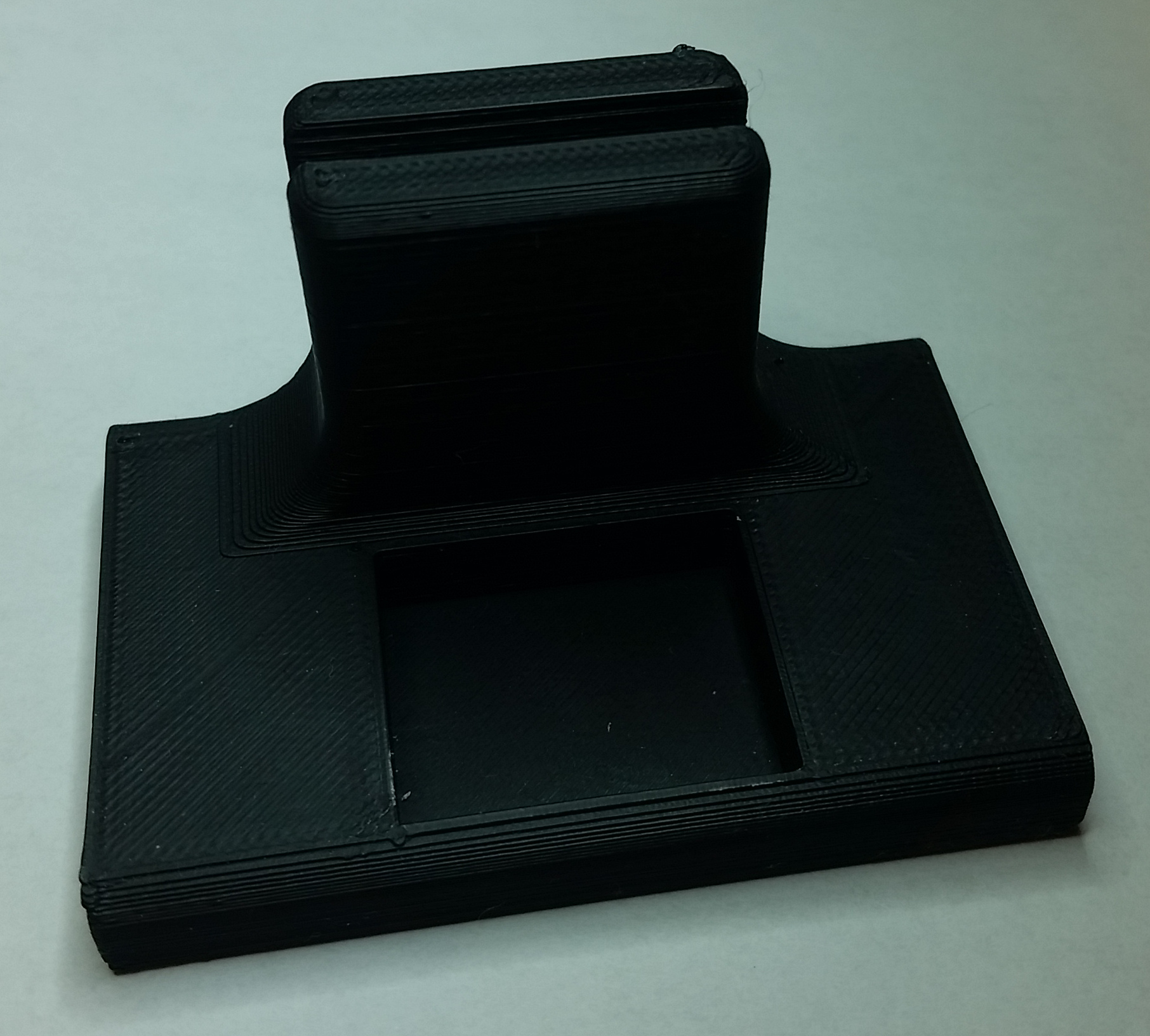
I printed this upside down to avoid requiring any support material.
Then I 3D printed it, screwd in the antenna, and hot glued on the magnets.
The print actually has a slight error about halfway through, but the tolerance on the magnets was enough that it was still usable.
I recently completely encircled my room with LED strips; in this post, I’ll outline how I set everything up.
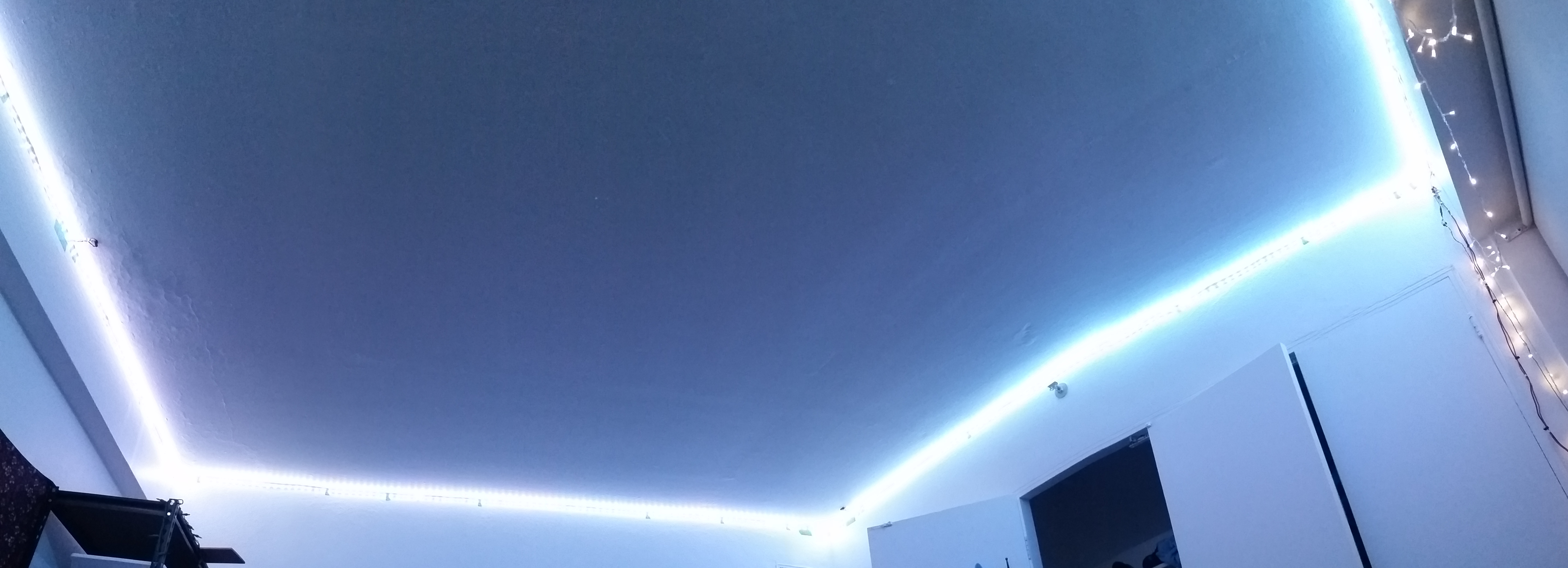
Here’s a panorama of the LED strip that forms a full loop around my room. The rainbow effect is a result of the entire strip fading through several colors in the time that it took to take the panorama. However, this strip is also addressable in triplets.
First of all, I used some low-LED-count strips with WS2811 driver chips, addressable in groups of 3 LEDs. Nowadays, you can buy very LED-dense strips that are truly individually addressable, but I knew that the triplet-addressable format was common a few years ago and conjectured that there would still be a few of these strips for sale on the cheap as manufacturers tried to sell off their remaining supply. I was right! I bought 16 feet of LED strip and ended up using most of it. I used the rest to illuminate my closet, which I’ll describe in a later post.
First, I set up the electronics, largely based on Adafruit’s guide here. The electronics consisted of a single several-meter LED strip, a 12V power supply, and a Raspberry Pi to control the strip. The Pi uses 3.3V logic levels while the WS2811 drivers on the strip use 5v to 12V, so I integrated a level shifter (the 74AHCT125) into the cable between the Pi and the strip, as shown below. I got a 12V power supply from re-use.
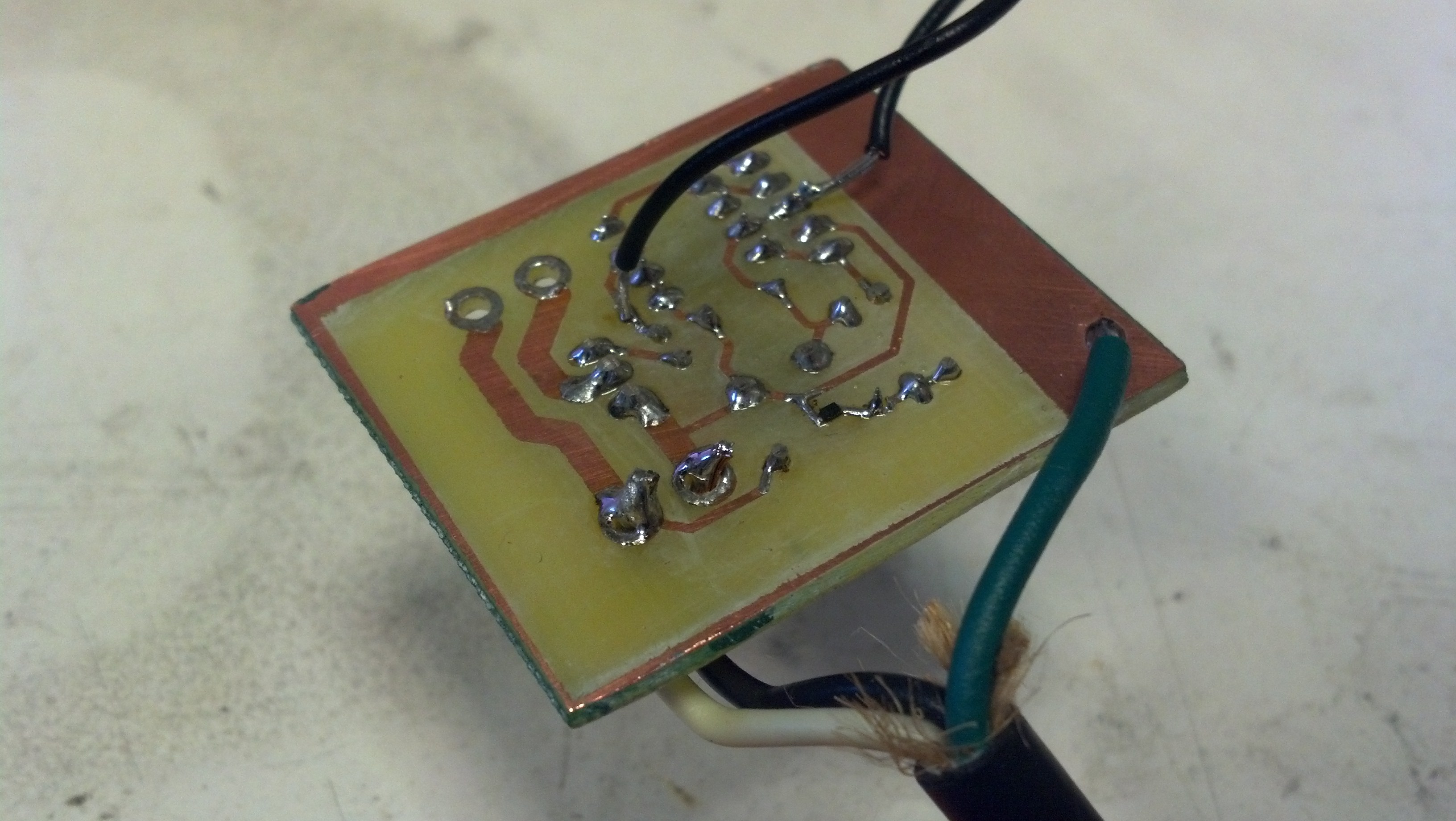
Check out my dead bug soldering.
After I set up the electronics, I mounted the strip to my wall. I was hoping to be able to use the adhesive backing on the strip, but it proved woefully ineffective, falling down after a couple hours. So, I temporarily reinforced the strip with masking tape and then developed some mounts to hold down the strips, as can be seen in the following pictures.
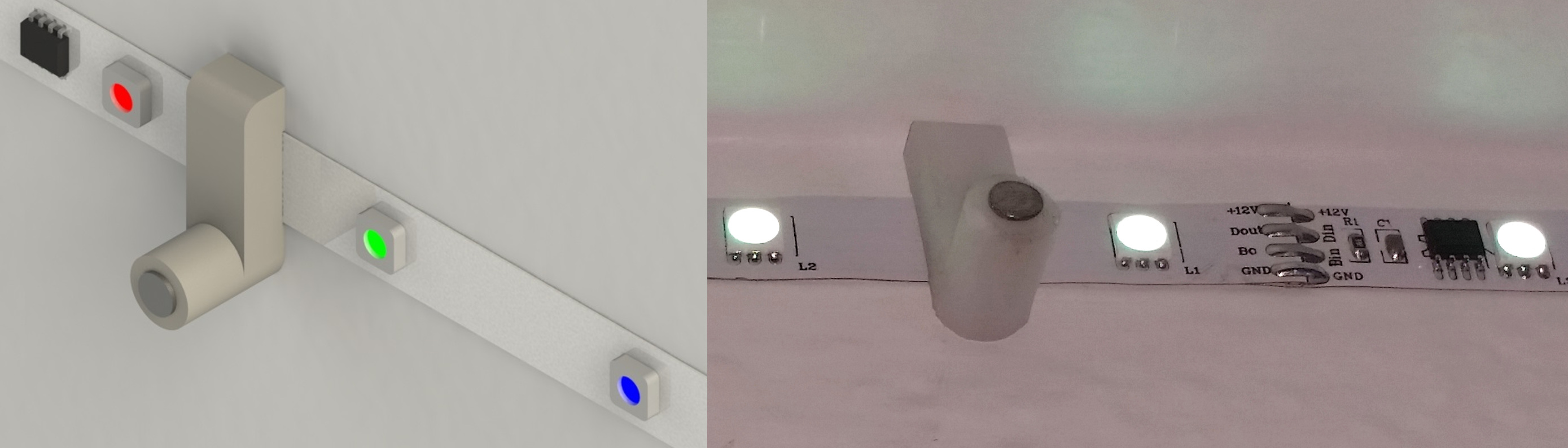
I could find similar LED strip clips online, but only with screw-sized holes. I wanted to use small nails for drywall, so I design and printed a nail version: rendering on the left, in place on the right.
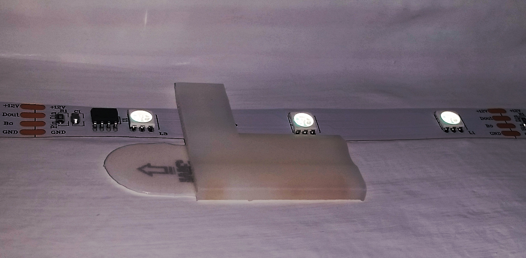
After mounting the strip on two walls, I realized that the other two walls in my room were actually concrete beams at the height of the ceiling. I can’t nail into concrete, so I whipped up a new version of the clip with a large pad for a command strip.
One problem occurred when I attempted to use the strips to illuminate my room with white light at maximum power: the color at the end of the strip would be much dimmer and redder in color than at the start the strip. I didn’t take a multimeter to it, but I expect the voltage at the end of the strip was drooping signficantly even while the beginning was at 12V due to the accumulated resistance over the length of the strip.
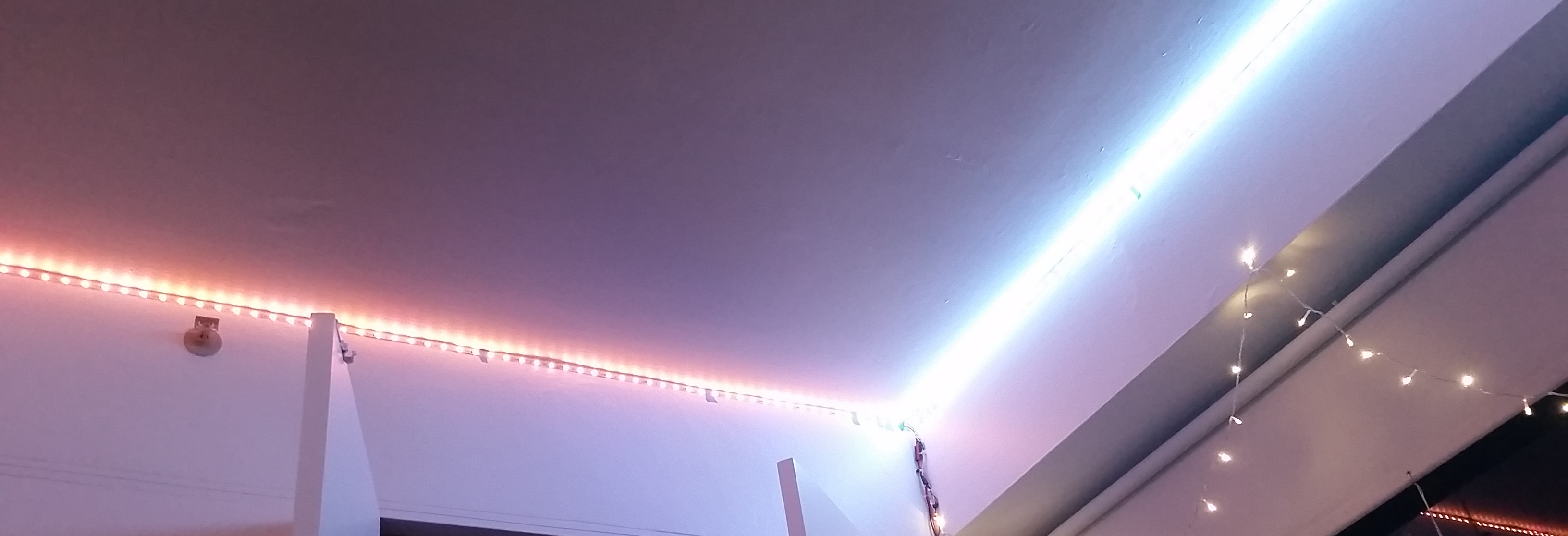
At this corner of the room, the strip starts (on the right) and ends (on the left).
I mostly resolved this by linking the power lines from the end of the strip to the power lines at the beginning of the strip in the corner where they met.
After applying the fix, the discoloration in the start/end corner (on the right) is nonexistent, and the discoloration on the far corner (bottom left) is minimal.
Subsequently, there was still a slight discoloration in the middle of the strip, in the corner of the room farthest from the beginning (and end) of the strip, but I resolved this (not pictured) by slightly dimming all the LEDs and then compensating the LEDs by a linear factor based on their distance from the start/end corner.
I run various effects on my strip that are only achievably with addressable (groups of) LEDs–theatre chase patterns, racing blobs of color, etc–but one of my favorites is simply running the same color on every LED and fading through the rainbow. This produces an effect on my other decorations, seen below, reminiscent of what I’ve heard called RGB Art. Here’s a gallery of RGB Art by artist duo Carnovsky.
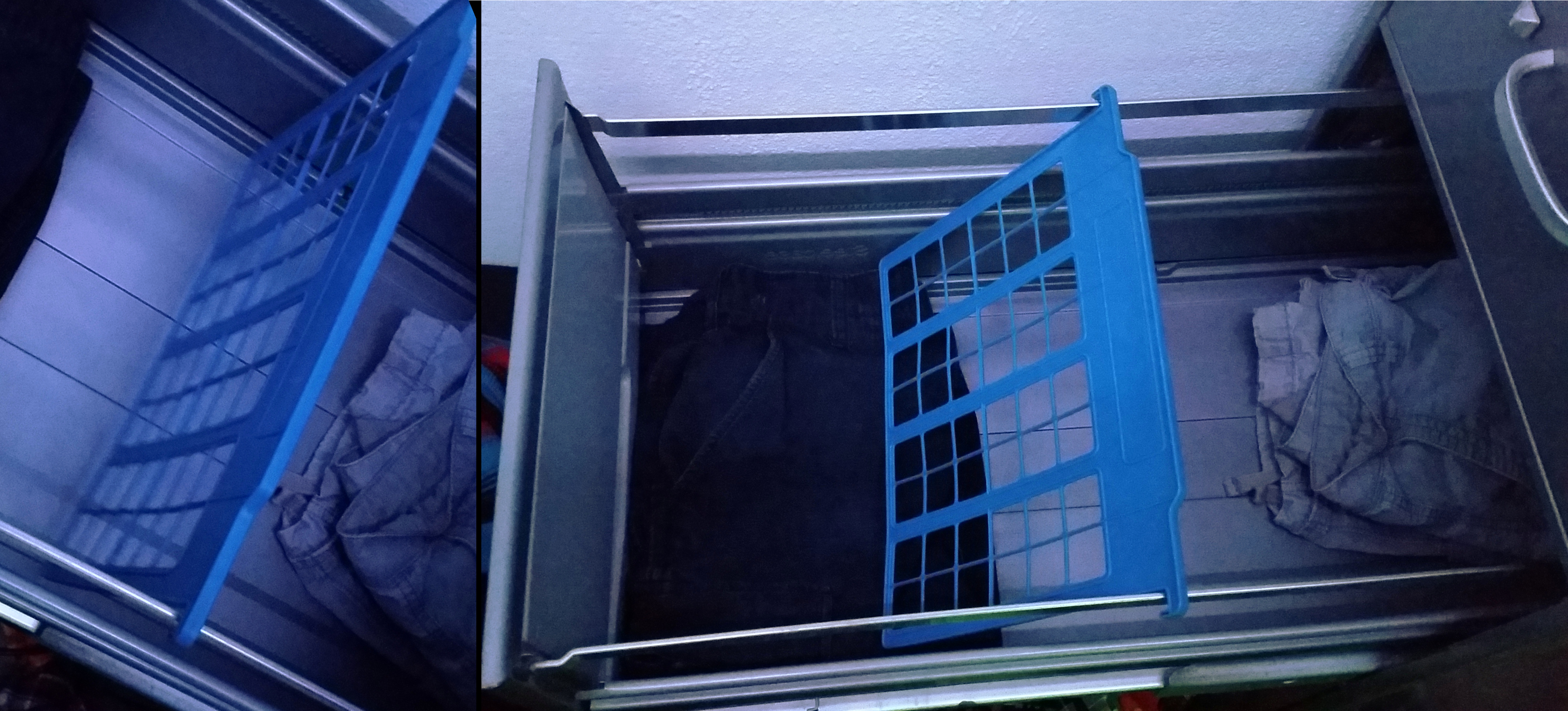
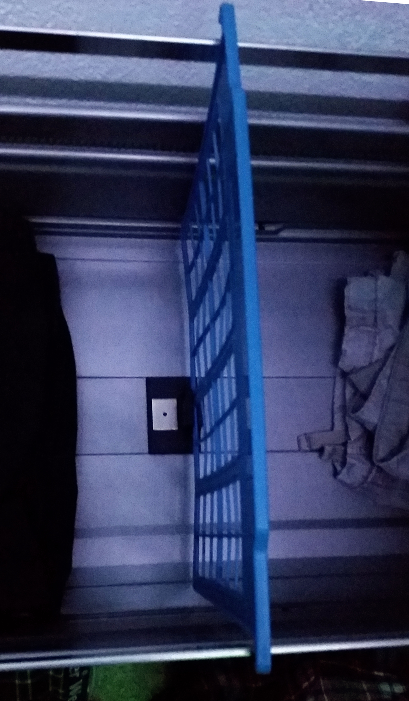
Quick part I made the other day: I keep my clothes in a filing cabinet, and I ordered some of these filing cabinet dividers the other day to divide some of the drawers into sections. Unfortunately, I ran into a problem where, as I shuffled around the contents of the drawers, the dividers would tip over since they weren’t actually mounted at the bottom.
Can’t have pants mixing with shorts!
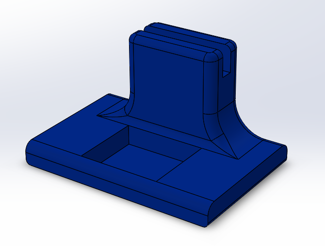
So, I whipped up a quick part to fixture the bottom of the divider to my cabinet.
I designed this clip to avoid any features that would catch on clothes. All the edges have large fillets, and the surfaces of the part are flush against the surfaces of the filing cabinet where it is inserted.
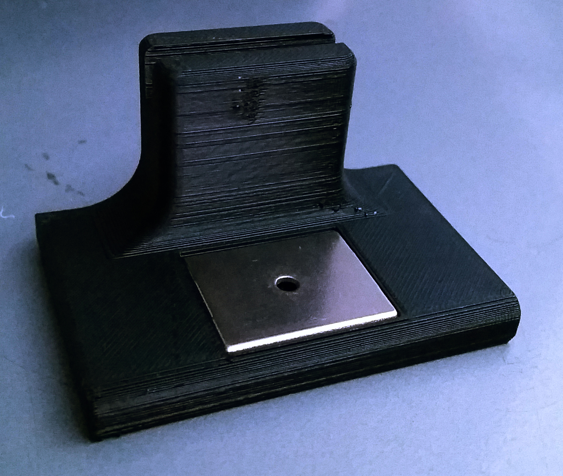
I used a 3D printer to print a couple. The divider interfaces with the part with a little bit of friction in the slot. A magnet (one of these) sits in the square cutout in the part and holds the part against the metal bottom of the drawer. The part sits in the channel in the bottom of the drawer.
Fresh out of the printer
The magnet surface is also flush against the surface of the clip.
As you can see, problem solved!
I printed a couple of these, one for each divider.
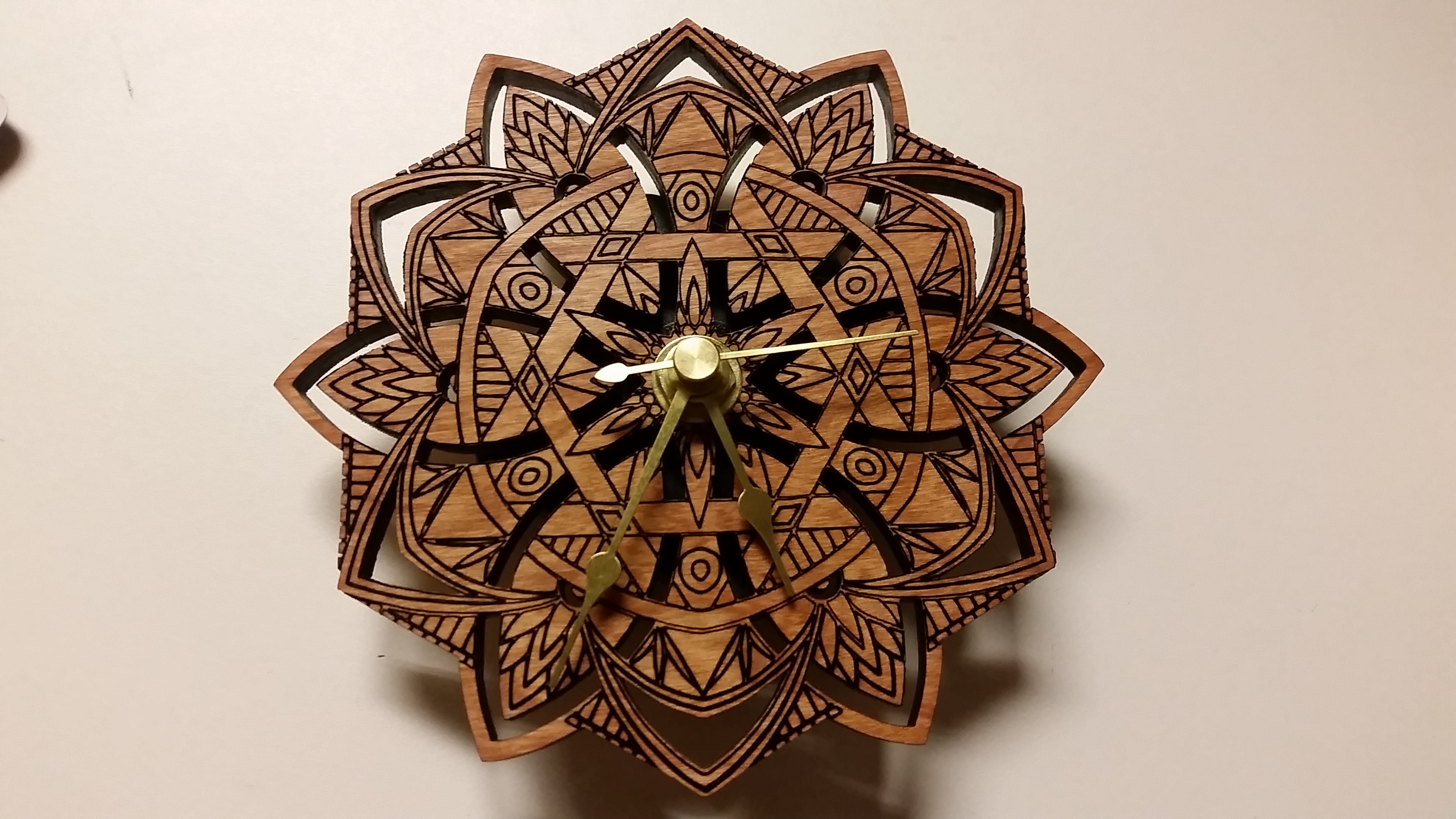
Here’s another relatively artistic project. I made this clock as a gift for someone:
Laser cut clock with a 12-point mandala face
The build was pretty straightforward. First, I searched online for mandala designs, and I started with one that I liked. The hardest part of this stage was finding designs that were 12-pointed; most mandalas have a 2^n number of points.
Next, I used Inkscape to vectorize the mandala and modified it to be appropriate for laser cutting. This included selecting parts to be engraved and cut as well as some tweaks to the design. I like making renderings to give me an idea of what the final project will look like, so I added some additional layers and a woodgrain bitmap to produce this preview.
This image gives a picture as to what the mandala would look like before laser cutting; I could use the same technique to visualize other designs cut and etched in cherry wood.
Satisfied with the design, I purchased some 1/4″ cherry wood and lasered it out.
Before cutting, I covered the piece in masking tape to protect the finish. It was a pain to remove the masking tape from all the little regions, but the result looks good. You can still see a piece of tape on the piece in this picture.
I think settings on laser cutters always take some tuning, so, for reference, I used these settings on a 30W laser cutter.
Cutting power: 100%
Cutting speed 32%
Cutting frequency: 2500Hz
Raster power: 25%
Raster speed: 100%
Raster resolution: 500dpi
Next, I applied linseed oil to the result. I bought a small clock movement with brass parts, which I inserted into the hole in the face.
My favorite part is how the color changes depending on whether you’re looking at it along the grain or against the grain. One way, it looks golden, and the other way, it looks reddish in color.
Hiya! I haven’t made any posts recently, so I’ve got a backlog of a couple projects to write about. Besides personal projects, I’ve also had a lot of life updates in the past year. First, I graduated! I interned at two companies, and now I’m back at school, working on a master’s program with the Biomechatronics Group.
In contrast to all these technical endeavors, I thought I’d start off with some relatively artsy projects.
Recently, I’ve been learning to spin fire fans. A video speaks a thousand pictures, so here’s a video from my very first fire fan performance, at Steer Roast 2016. Credit to Ivan F for the video.
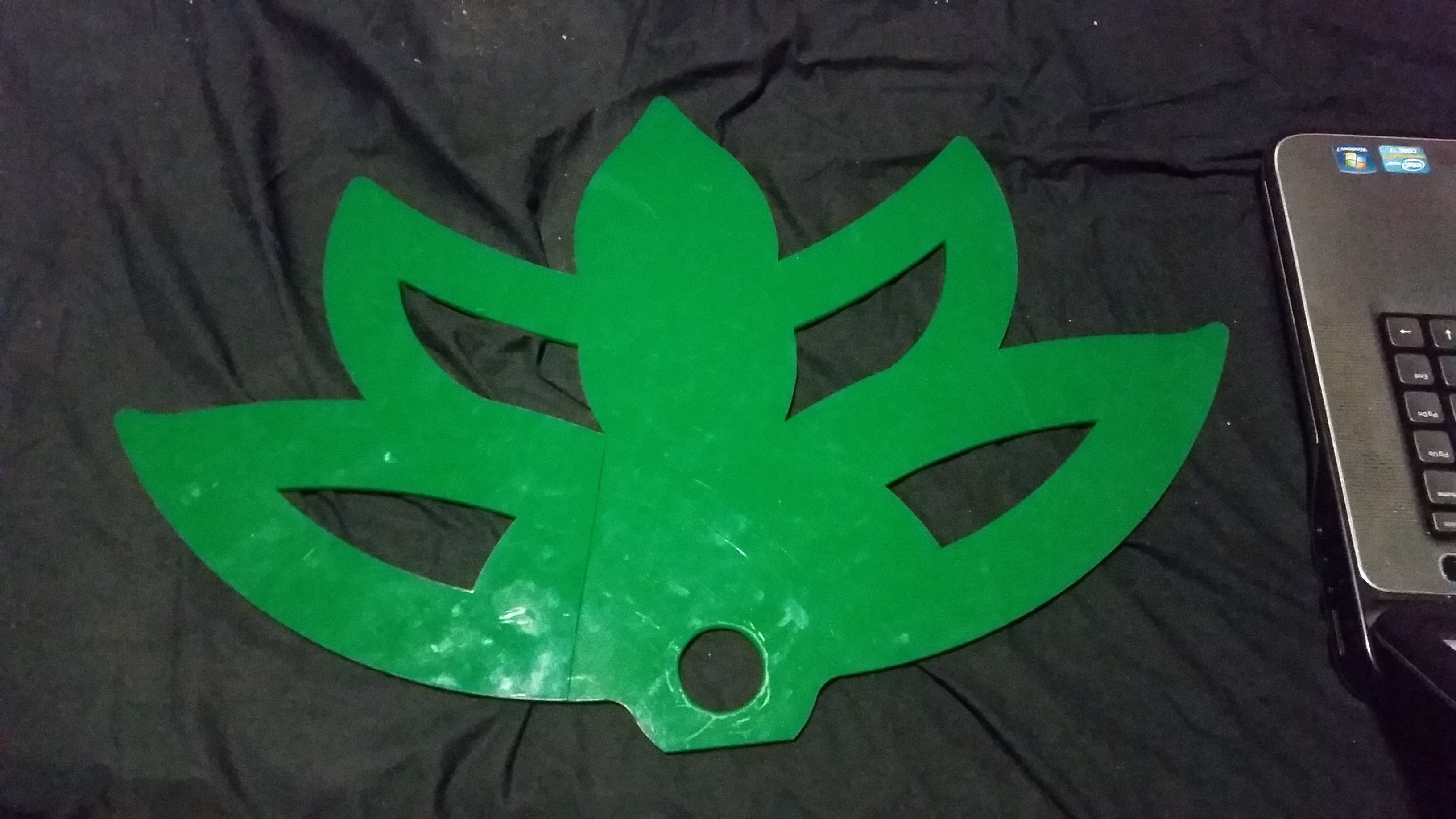
Prior to getting fire fans, I wanted to build some practice fans. Here’s my first prototype:
Here’s my first prototype, cut out of green acrylic.
I sketched up a lotus shape in solidworks and cut the shape out of 1/4″ acrylic with a laser cutter. Acrylic is not the appropriate material for the final application — you can see this fan already has a crack in it, but I wanted something to play around with first.
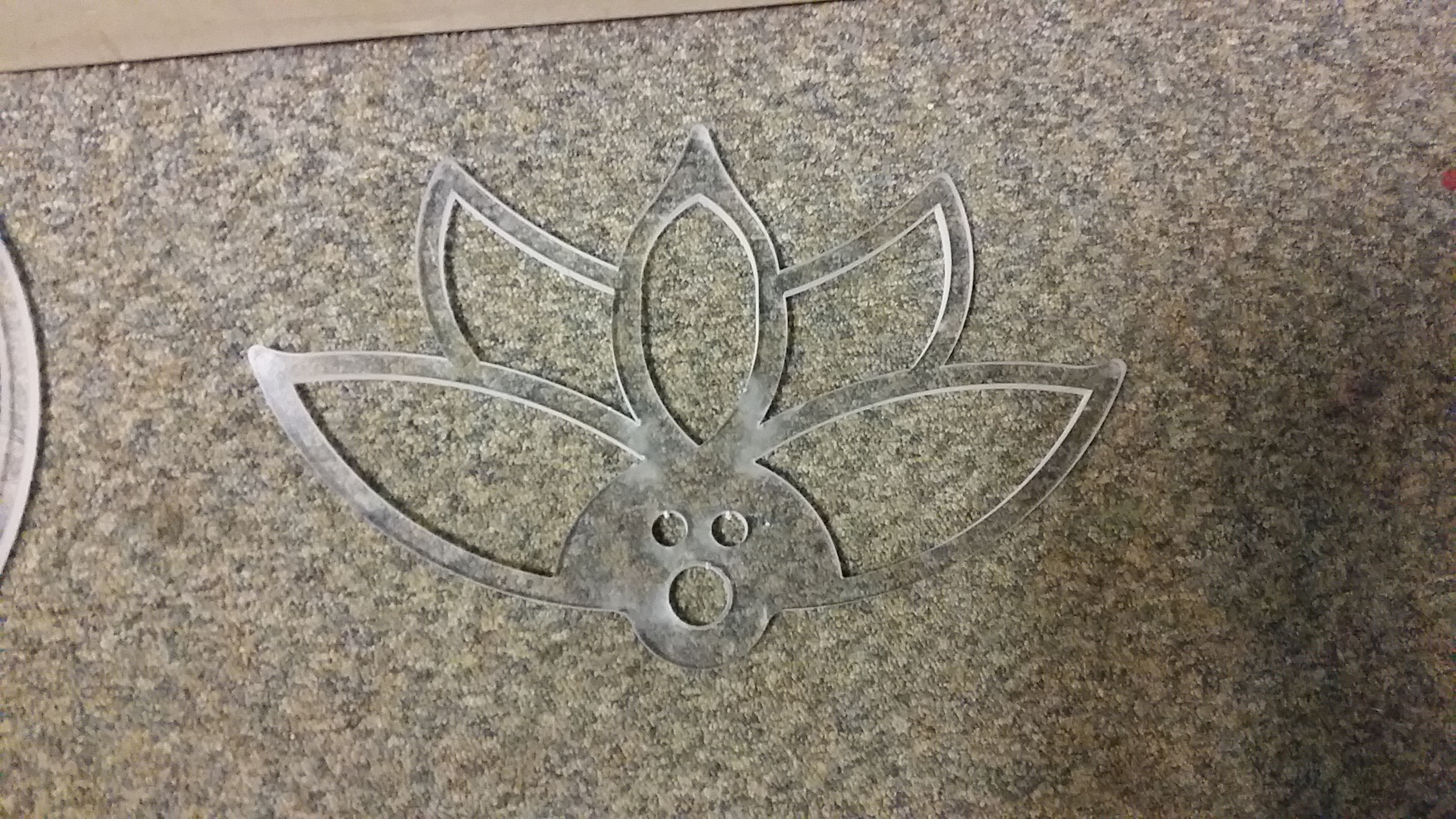
Based on this version, I changed some thicknesses and cut new fans out of 1/2″ clear polycarbonate. The polycarbonate is more appropriate for the impacts that I expect these fans to take. I got polycarbonate from a lab cleanout on campus–the sheets used to be splash shields for some kind of chemical process. I used a waterjet to cut out this version
I sanded down the finger hole in the middle to be more comfortable
Now that I have some fire fans to compare the weight with, I’ll make some more modifications. One popular choice of material for practice fans is HDPE for its slickness. Indeed, the polycarbonate fans I made are rough on the hands. However, HDPE is very brittle for this application. I’m considering making polycarbonate fans with press-fit HDPE finger rings for my next version. I also like how the polycarbonate is translucent–I’m considering inserting LEDs in my next version to made a rave-ready pair of practice fans.
What do you think would be good features in fans like these?
Following up my last post, I took another Introduction to Robotics class last semester, but this time it was the Mechanical Engineering department’s 2.12, which goes into more depth on the modelling and control of robotic mechanisms. See my previous post for a quick comparison of the classes.
Instead of exploring an environment and building a structure out of blocks, the final project for 2.12 was a little more constrained. The final project was the World Cup of robotics, a soccer competition to be played by the robots of the class. The class was divided into several groups, each representing a nation, and each group fielded a goalie robot and a kicker robot. A team of three other undergrads and me, dubbed “Team Kicking and Screaming” built the kicker robot for our nation.
Here, you can see our final robot in action. The robot uses data from a camera system to predict the ball’s motion. With this model, it then calculates the point in time and space at which the ball will intersect the workspace of the robot. When the ball is close enough, the robot starts a kicking trajectory such that the shoe will meet the ball at this point in time.
In order to implement this behavior, we wrote several software modules. These included a module for accessing the camera system, a module for predicting the path of the ball, and a module for inverse kinematics and motor control, among others.
For vision, the 2.12 TAs set up a computer to extract the ball coordinates from a ceiling-mounted camera using techniques we studied in an earlier lab assignment. The machine published these coordinates to a TCP server with updates promised roughly 60 times a second. We first wrote software to poll this server and to perform calculations with the data.
Next, we got to work with ball trajectory tracking. We were writing software at the same time as the TAs were setting up their vision software, so we weren’t able to immediately test different models of rolling ball motion using real data. With this in mind, I deliberately left the model as a parameter that could be supplied by the user, and I used the curve_fit method of SciPy’s Optimize module to fit the data to whatever model was supplied. This method uses the Levenberg–Marquardt algorithm for curve fitting, which can be applied even for non-linear curve fitting.
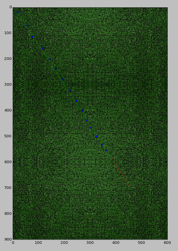
Written before the camera system was set up, a piece of our software software generated the following demo image. Upon being fed coordinates that represent sampled locations of the ball, plotted in blue, the software adjusted parameters to fit a trajectory model, and it plotted the calculated trajectory in green. The red line is the software’s prediction of the future path of the ball if it remains on this trajectory. The sample points were broadcast from a server hosted locally and were deliberately spaced far apart for ease of debugging, but the actual data would be more dense spatially.
Our software fit the above trajectory to the blue points as they were published. The axes are measured in pixels; the resolution of the field is roughly 2.5px/in. Once built, the actually field was a little smaller, and ball coordinates were published much more densely.
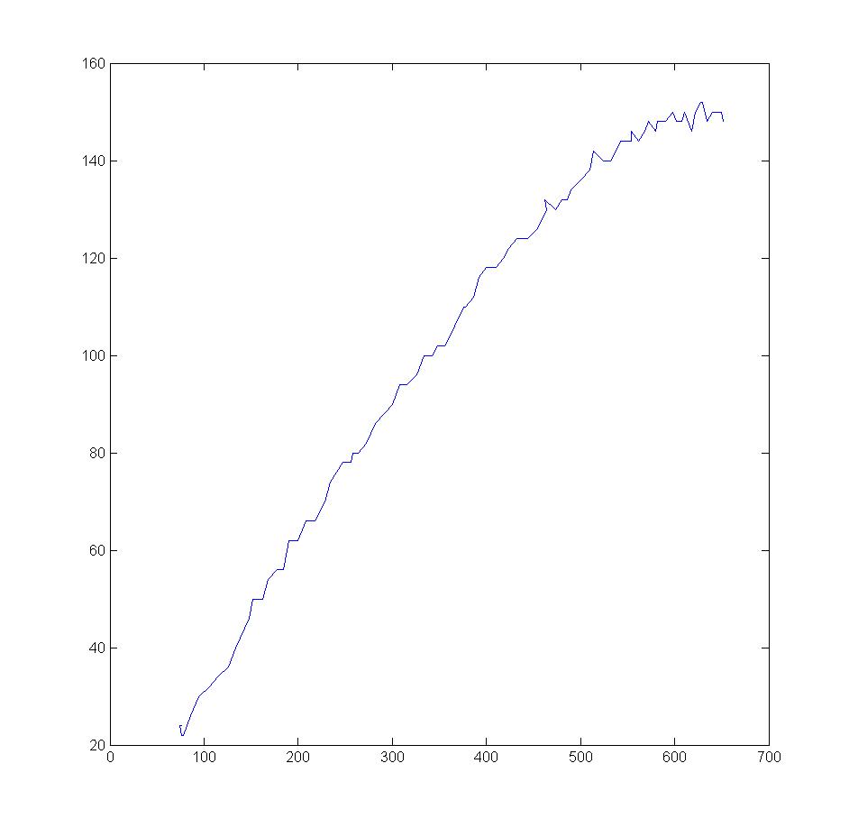
Once the field and camera system was set up and we observed the movement of the ball, it became apparent to us that the a good model of ball motion could indeed be nonlinear. As the ball slowed, the general curvature of its trajectory often increased. More significantly though, being a buckyball-shaped soccer ball, the ball would wobble from side to side as it landed on different faces of its surface. This motion was on the order of inches.
This plot of a ball’s motion over the field coordinates, captured from the field vision system, demonstrates the wobbliness of the ball’s motion as it slows down. The ball entered from the lower left and rolled to the upper right. Both axes are in pixels at roughly 3.5px/in. This plot is deliberately compressed to make the curvature more apparent.
Luckily, as the project progressed, it became apparent that they intended to roll the ball at a higher speed than what we were initially testing. At higher speeds, the wobbling effect was diminished, and we were able to use a relatively simple model of a rolling ball with rolling resistance.
Once we had this ball trajectory, we wanted our robot to be able to predict at what point the ball would intersect the workspace of our robot. At this point, unsure of what ball trajectory model we would use, we were faced with the problem of finding the intersection of two arbitrary curves: the trajectory of the ball, and the perimeter of the workspace of our robot.
Our solution was to discretize each curve as a finite number of line segments and then iterate through them until an intersection was found–this way, we could make a trade-off between the spatial resolution of the intersection point and the amount of time to compute the point. This strategy finds the intersection point, if there is one, as long as the line segment lengths are small compared to how far the path can diverge from a straight line approximation over a single discretization step. In our case, the inertia of the ball limits how far its path could diverge from a straight line.
It turns out there aren’t many computational geometry modules available in Python, so I ended up writing my own to evaluate whether two line segments intersect. I’d be happy to hear if I overlooked something, so let me know.
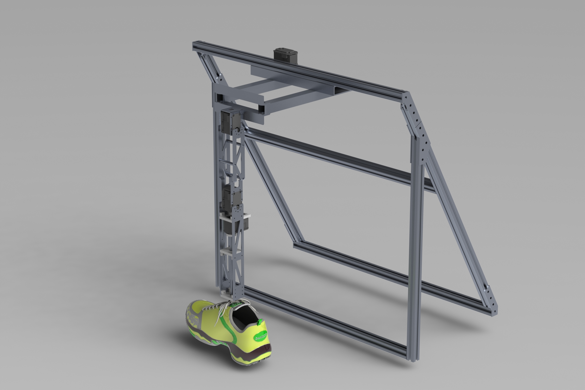
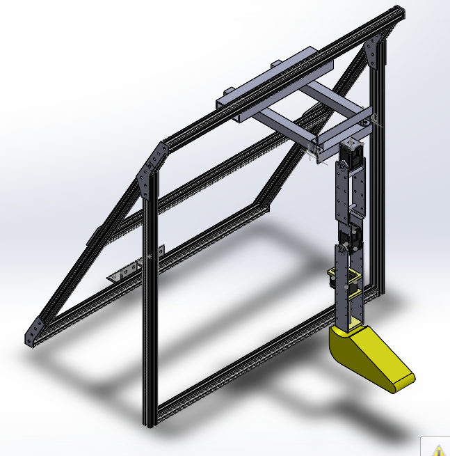
The other members of my team developed the hardware for the robot, though I waterjetted some parts. The result of their design was this super kickass leg, as you can see from these renderings.
The frame of the robot attaches to a baseplate on the field while the leg terminates in a shoe to interface with the ball.
Once we developed the design for our robotic manipulator, we performed wrote software to perform inverse kinematics with the parameters for our robot. With this kinematic model available, we wrote software so that that our leg would follow a trajectory, ending at the time and space when the ball intersected our workspace.
The lowest motor in this rendering adjusts the yaw of the ankle of the robot. Above this is a motor for controlling the angle of the knee, and above this is a motor for controlling the angle of the hip. The entire leg can move side-to-side, tracing out a semi-circle, using the driven parallel linkage between the hip and the frame.
Here’s the github repo for our code, which might be helpful for future teams. We wrote the majority of our code in Python with SciPy for curve fitting; and we used MATLAB and matplotlib for graphs.
Ok, this post is about catching up on an old project!
A semester ago, I took MIT’s Robotics: Science and Systems (6.141). I feel obligated to mention that, sadly, the instructor of this course Prof. Seth Teller has since passed away. On this topic, the MIT news office has a well-written article on Prof. Teller and his work. However, the focus of this post is going to be on the structure of the course and the final project.
My team used a few techniques to build this robot quickly and flexibly for our final project for 6.141.
It turns out there are several introduction to robotics classes at MIT. 6.141 is offered by Course 6, the Electrical Engineering and Computer Science department. However, there’s also Introduction to Robotics (2.12), offered by Course 2, the Mechanical Engineering department. Last semester, I took 2.12, and it’s safe to say that both 6.141 and 2.12 offer a hands-on introduction to robotics, but from different perspectives. 6.141 has a focus on algorithms related to robotics, such as those for navigation, motion planning, and machine vision. By contrast, 2.12 has a focus on analyzing mechanisms, like multijointed robotic arms or legs. The two classes had some overlap in their discussion of techniques for sensor fusion and filtering. 6.141 also offers an introduction to the Robot Operating System (ROS) and has a technical speaking and writing component. As someone who is interested in improving my public speaking skills, I thought the speaking component was fun. For students interested in robotics, I recommend taking both.
That said, Course 6 also offers an EECS survey class, 6.01. Though I hear 6.01 has changed since I took it, I found it was also a great class in terms of introducing students to problems and algorithms in robotics, perhaps as good as 6.141. For example, 6.01 included a series of labs in which students wrote code snippets for filtering, state estimation, and path finding, which ultimately allowed robotic vehicles to race through a maze. Like 6.141, the labs in 6.01 seem to build up to the notion of SLAM, starting with labs on simple navigation techniques and gradually becoming more advanced. However, unlike 2.12 and 6.141, 6.01 lacks a final project component.
The final project components was also how 2.12 and 6.141 differed. Ironically, although 6.141 was a computer science class, and 2.12 was a mechanical engineering class, I found I did mostly mechanical work for my 6.141 team and mostly software for my 2.12 team. I suppose this is because 6.141 attracted mostly computer science students, and 2.12 attracted mostly mechanical engineering students. For this reason, though, I’ll discuss the mechanical design of our 6.141 robot here.
The final challenge for 6.141 was to build, in a team of five, a robot to explore a room-sized arena, find colored blocks, and build a structure with them. We decided a neat way to further define the problem would be to build several towers of blocks, with each tower formed by only one color of block. We were also pressed for time, so I took a few steps to build this machine as fast as possible.
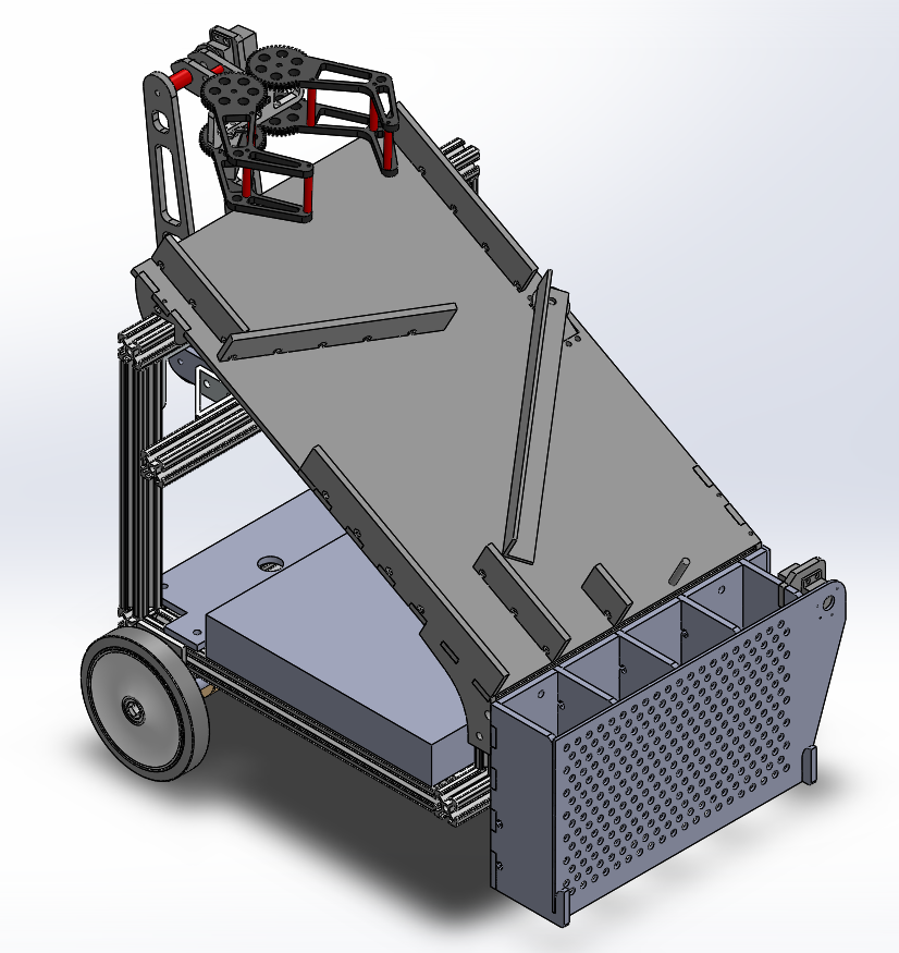
With this in mind, I decided the best way to design the hardware of the robot would be to break it up into physical modules. Each module could be designed independently, allowing people to design them in parallel, or at least reducing the cognitive load if one person worked on all modules. After consulting with the team, I settled on four: a chassis module, an arm/manipulator module, a block sorting module, and a storage module. The chassis would be the base of the robot and would include the frame, wheels, motors, battery, and laptop computer. The manipulator and arm would be mounted on the front of the chassis, able to pick up blocks from in front of the robot and drop them off on top of the robot. Atop the chassis would be mounted the block sorting module, which would sort and deliver blocks to the storage module, mounted to the back of the chassis. Finally, the storage module would feature a door or gate to release the blocks, stacked in tower formations.
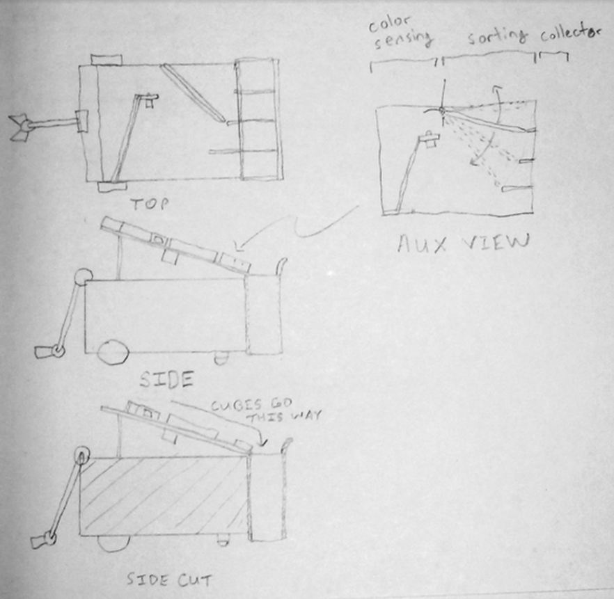
This initial sketch of the robot included a fifth module: a color detection module attached to the front of the sorting module. However, we later decided to mount the color sensor on the claw itself, eliminating the need for color sensing while chanelling blocks.
Another convenience about the modular design of our robot was that it was really easy to take modules on and off. For example, to get at the electronics of our robot, mounted on the chassis, we could simply unscrew two screws and lift off the sorting mechanism.
So that I could design each module separately, I first settled on the interfaces between the modules: each module would be able to attach to a separate horizontal bar of 80/20 aluminum extrusion attached to the chassis. I knew that I would want to adjust the exact heights and other dimensions of each module after I built the first prototype, so I deliberately designed these 80/20 bars to be adjustable in a few dimensions, such as height. Also, using the same technique as I detailed in my post about a window fan, I created a dimentions.txt file in which I recorded these dimensions. I used these as global parameters, which I referenced while designing each module, knowing their specifications for the connection points were the interfaces between each module.
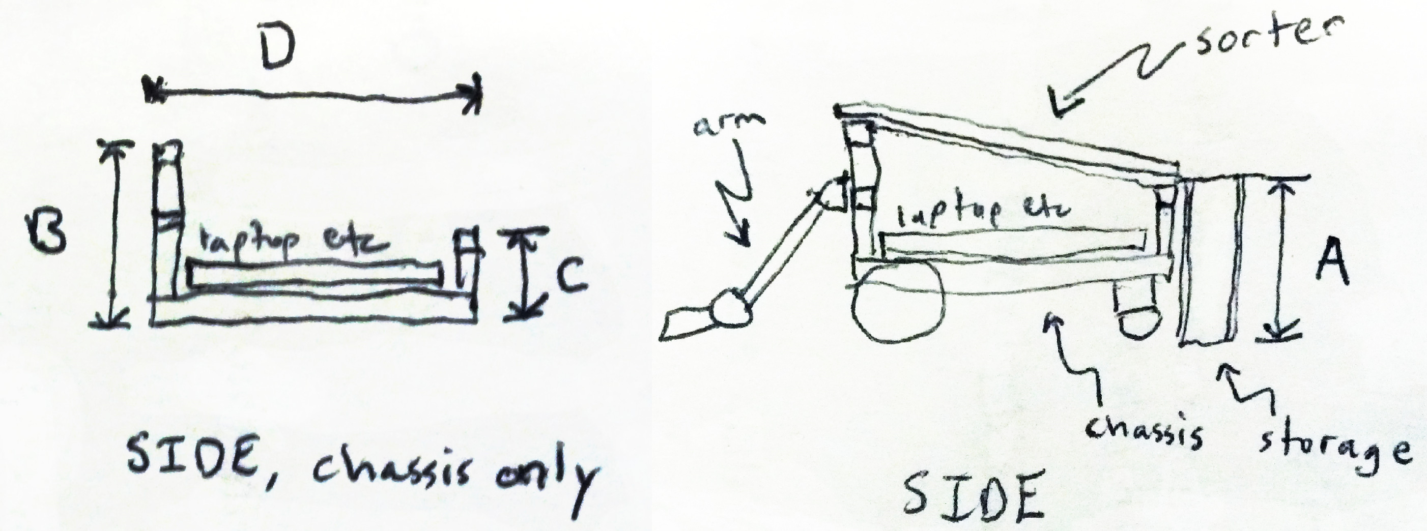
At the start of creating CAD for the robot, I created a quick drawing to specify the meaning of dimensions A, B, C, and D in this drawing. I gave them names and specified them in dimensions.txt.
Also to cut down on construction time, I designed each module mostly out of 80/20 and laser cut acryllic. Using the laser cutter made it easy and fast to cut improved versions of parts. I also used Jesus Nuts for fast assembly.
The first two modules were straightforward. The chassis I designed was a slight adjustment from the squarebot chassis we had been using in labs earlier in the semester. Similarly, the arm and manipulator were re-used from earlier labs, but we added a color-detecting sensor to the manipulator to detect the color of the block being grasped.
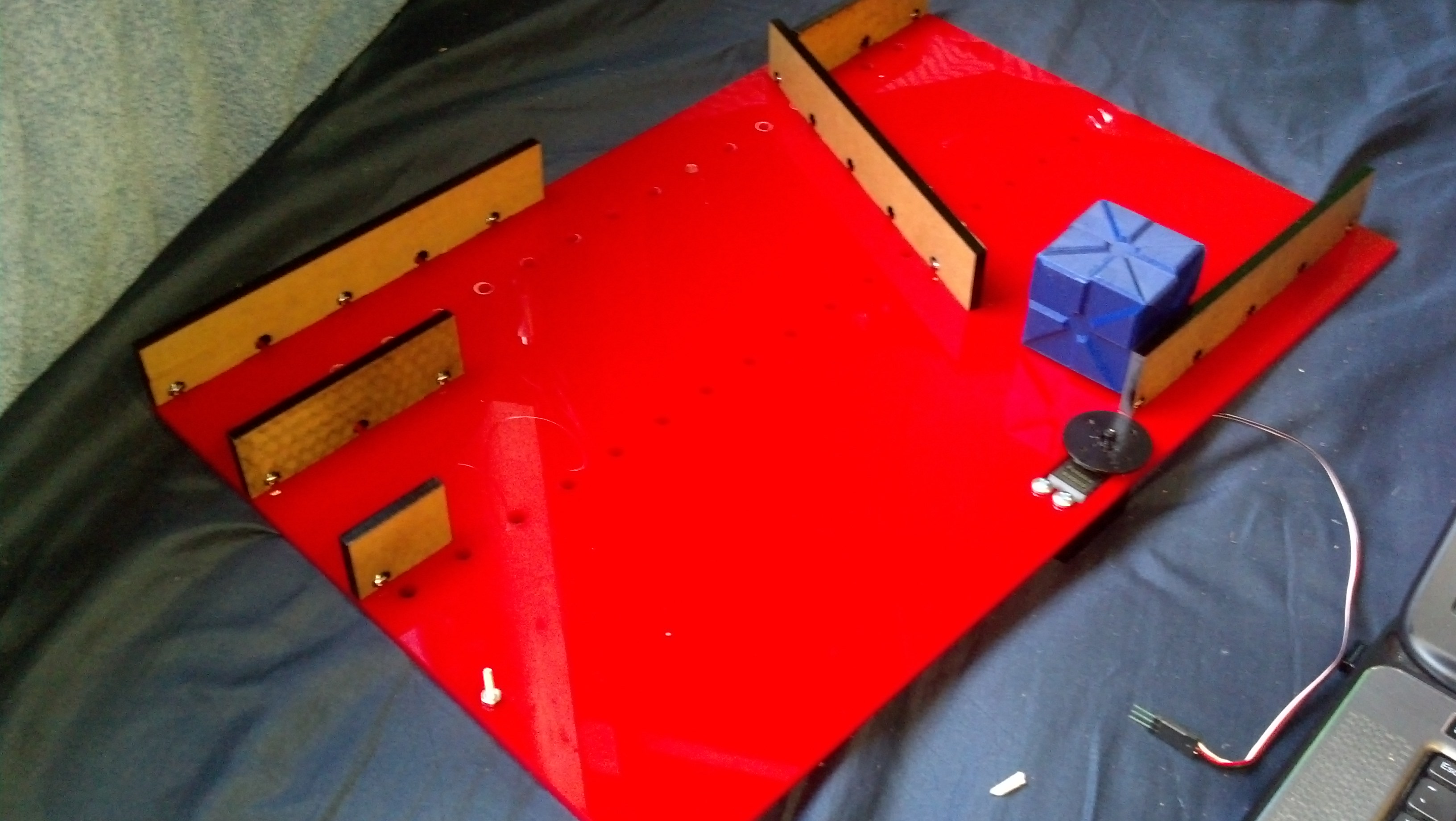
For the sorting module, we came up with a few options but settled on one that minimized the number of moving parts. The module consisted of a slanted panel with guides for blocks. First, the manipulator drops blocks off at the top. Then, one guide funnels all the blocks to one side of the robot. An actuated flipper then guides a block to one of four channels depending on the color of the block determined earlier from the color sensor.
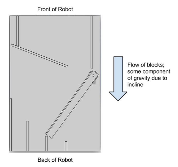
This view, normal to the surface of the sorting mechanism, shows how blocks are first funneled to the flipper then channeled to a chute. Gravity pulls them down the mechanism.
The first version of the sorter mechanism was fast to assemble and convenient for testing things like the minimum slope required for cubes to slip.
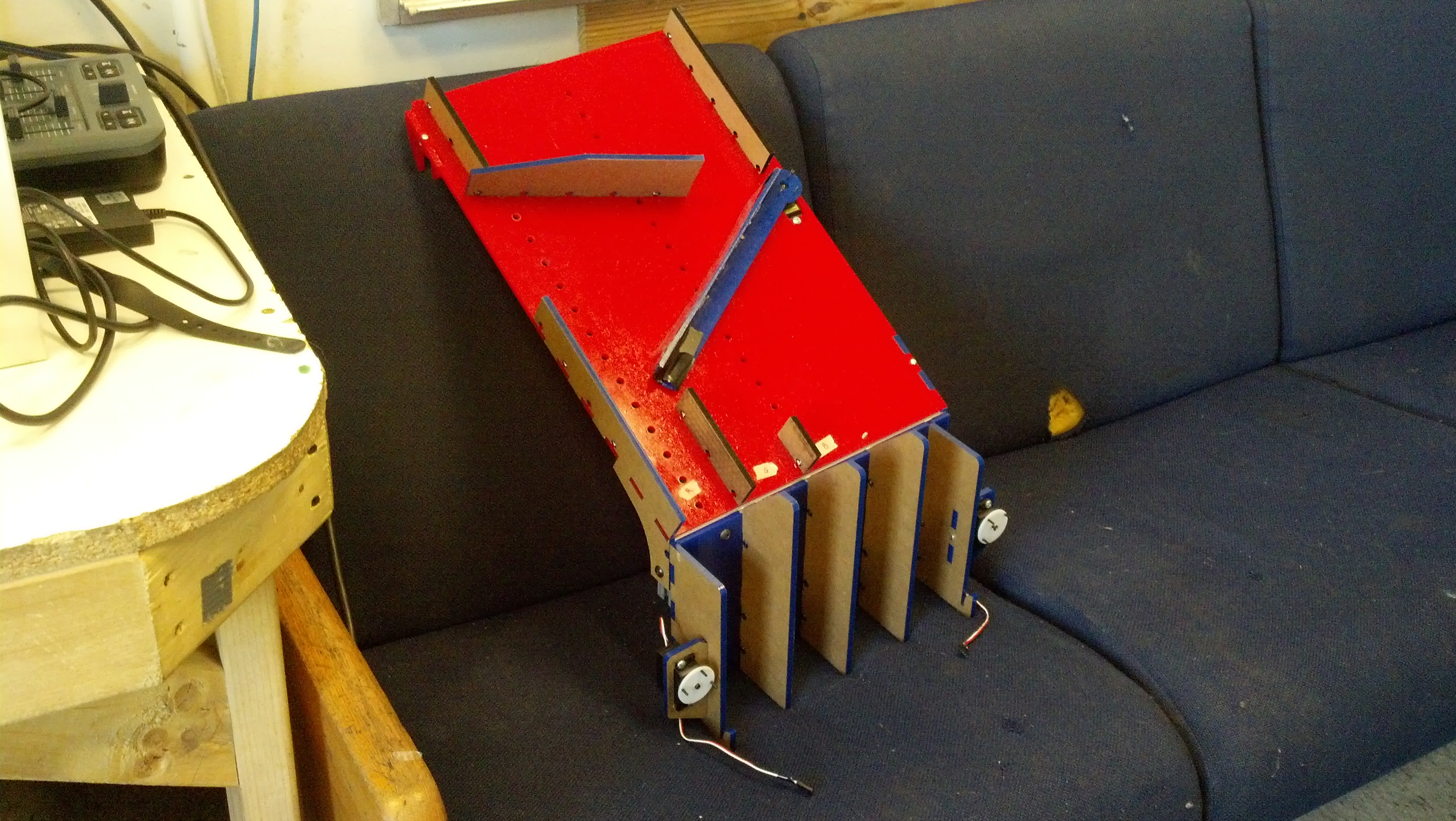
Finally, the collector module consists of four containers just big enough for cubes to stack one atop another. I created a few prototype single-column containers to determine the amount of extra room necessary to keep blocks from sticking to the wall. The containers were open on the top to allow blocks to slide in from the sorting module. I designed one side of the module to open, allowing the robot to drive away, leaving four towers of stacked blocks.
The final storage mechanism included four columns and a double door at the back. Here, the doors are removed to see inside the chutes. The final sorter module is also attached atop.
As mentioned earlier, these techniques allowed me to quickly make improvements to parts. For example, I increased the heights of certain walls that blocks were able to fall over, I increased the slope of the sorter to reduce the chance of blocks sticking, and I replaced the single door on the back of the storage mechanism with a double door mechanism because the weight of a single door was pushing the limit of what the servo could provide.
Unfortunately, I wasn’t able to collect much video footage before the disassembly of our robots, but the following two videos show our robot during testing and in action.
Also known as the “Sketch as Fuck Lamp Dimmer” per my friend Eric, the design originating from this application note in general has the usual lamp dimmer topology: a zero detector, a timer, and a triac. These three components implement phase cutting, specifically the triac performs phase cutting on AC current from mains supplied to a load. The first two components, the zero detector and timer, are both implemented in a microcontroller, the subject of the application note.
However, this circuit is unusual in terms of its logic power supply, whose ground is not connected to the neutral of mains. Rather, the 5V node is connected to the hot wire of mains, and the 0V node is constructed 5 volts below that wire.
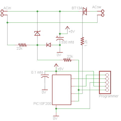
I designed my schematic in Eagle. Though not labeled, for space, the diode is a 1N4448, and the zener is a BTZ52C5V6T-TP.
One consequence of this is that, while plugged into mains, the logic of this circuit cannot be connected to any logic that is grounded to the neutral of mains unless the signals have some isolation. For example, I couldn’t connect connect my PIC programmer to the circuit while the circuit was plugged into mains without something exploding! To get around this, I plugged my circuit into an isolation transformer prior to mains during the latter part of programming the circuit, after I had confirmed my circuit functioned correctly electrically. As discussed later, this design is necessary to achieve proper biasing in the circuit, and you can see this power supply in other circuits as well–for example the application note for another lamp dimmer from ST.
Amused by this application note, I decided to build my own programmable lamp dimmer circuit. There are a couple neat techniques I took to make this project, so I’ll go through them one by one.
Power Supply Component Sizing and Theory of Operation
The application note intends to point out the low power consumption of the PIC10F microcontroller. As an example, it suggests building a lamp dimmer whose logic power supply resembles a 5V linear zener regulator. The power supply schematic from Eagle is given below–the 5V and 0V nodes are the power supply for the microcontroller. Normally, a linear regulator is not appropriate for converting between such disparate voltages — 120V (rms) to 5V. The voltage change is implemented by dropping the difference in voltage across a resistor, the 22k resistor in this case. Really, the only advantages to this kind of circuit are the relatively low number of parts, the cheapness of those parts, and the small footprint of those parts. For example, a circuit of components of this size could be embedded in the plug of a lamp itself, perhaps as a feature or a prank.
This regulator converts mains 120VAC to 5V; mains is plugged into the connection indicated, with hot connected to the upper wire and neutral the lower wire.
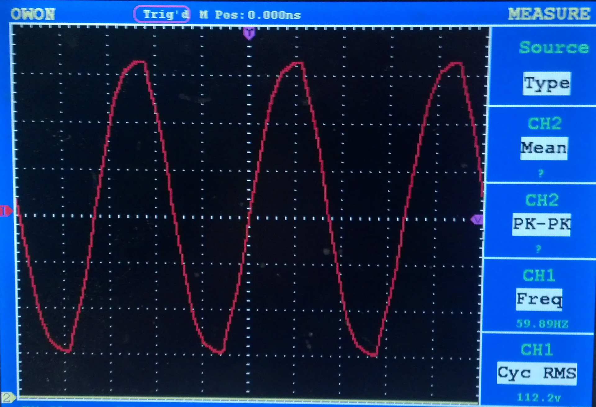
To explain how this circuit works and how to size components, let me simplify it. First, let’s consider the AC input signal, which is a hot wire and a neutral wire whose voltages differ by a 120VAC sine wave. An oscilloscope reading I took of mains is shown below.
The resolution is 50V/div. Mains provides roughly a sinusoidal waveform.
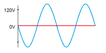
However, since what we intend to be the 5V node of the power supply is connected to hot, let’s instead consider the relationship between hot and neutral with hot as our reference voltage. This is still a sine wave, we’re just using neutral as our fixed reference, as shown in the following plot, where neutral is blue and hot is red.
Neutral is in blue and hot is in red.
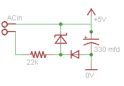
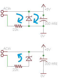
The rectifier diode (the non-zener diode in the circuit) may make this circuit hard to understand for someone who understands a regular zener regulator, so let me replace it with an ideal diode with no diode drop–it conducts like a wire when it is forward biased and does not conduct when it is reverse biased. Then, the circuit is always one of the two circuits in the following image.
This image shows two circuit representations if the diode were replace by an ideal diode with 0V forward voltage. The 0V forward voltage is inaccurate and is close to 0.7V, but in the actual circuit, the zener diode compensates for this because it is not actually a 5V zener but close to 5.6V.
During the first half cycle of the plot of neutral above, when neutral is negative with respect to hot, the diode conducts, so current flows from hot through the zener, capacitor (until it charges), and system load. Then, the sum of these currents flow through the 22k resistor to neutral. Due to its conduction characteristics, the zener diode drops at most 5V, and so the capacitor charges up to this voltage. The zener was selected specifically to have a low required zener current (on the order of 1 mA). The 22k resistor was sized to allow enough current for the system to run and the zener diode to zener while limiting the current to be less than the amount that would destroy the zener.
During the second half cycle, neutral is positive with respect to hot, to the diode is biased in the opposite direction. Current still flows through the resistor, but in the opposite direction and back through the zener. However, current does not flow from mains through the capacitor or the rest of the system. Rather, the microcontroller draws current from the capacitor, and it slowly discharges. The capacitor was sized such that it could power the microcontroller for one half cycle without its voltage drooping significantly. The 330mfd capacitor chosen corresponds to a 10% droop. I later shrunk the capacitor, taking note that this particular controller actually runs on as low as 2V.
Notably, the resistor could actually be larger, as a 22k allows as much as 7mA, and at 22k, the resistor dissipates on the order of half a watt, more than ought to be dissipated by a quarter watt resistor. In my circuit, the resistor heats up considerably. In future versions, I’ll replace this with a larger resistor, such as 220k. The 22k size is an artifact from the size chosen in the original application note, which appears to be a typo. Equation 5 of the application note incorrectly comes to the conclusion that passing a 0.7mA current across a 110VAC drop requires a 22k resistance when actually this number is 220k. The application note also spreads the power dissipation across two quarter watt resistors.
Based on this explanation, we could imagine systems where it is not the case that logic 0V is disconnected to the neutral of mains. For example, we could rearrange the regulator such that the 0V node is connected to neutral and the 5V node passes through the 22k resistor to hot. However, then we would also have to place the triac below the load such that it is switching. As a result, we would be switch neutral rather than switching hot, which is undesirable because it breaks convention. Moreover, some two-terminal AC devices have their cases grounded to their neutral, so this is undesirable in terms of safety as well. Moreover, if one logic power rail (0V) is at the level of the triac, and the other is 5V above it, then we will be switching the triac in quadrants 1 and 4 rather than 2 and 3. Quadrant 4 of a triac consumes the most current, so we would prefer to avoid it. As a result, we construct a system where one logic rail (5v) is at the level of the triac, and the other is 5V below the triac.
Update: Zero Detector
Eric says I should write about the zero detector, too, so I’m adding a section here. He says:
cool
you didn’t talk much about the zero crossing detector which i think is almost as cool as the regulator
since you can’t just take 120 VAC and put it into a microcontroller pin
but they tapped it off the pre-capacitor regulator
Basically, the voltage at the node between the zener and rectifier alternates between slightly above +5V (due to the zener diode forward drop) and slightly below 0V (due to the rectifier forward drop). As a result, this a great node to use for zero crossing detection.
Etch Mask with Spray Paint and Laser
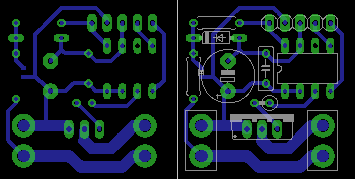
Left shows the copper traces while right includes an overlay of the components.
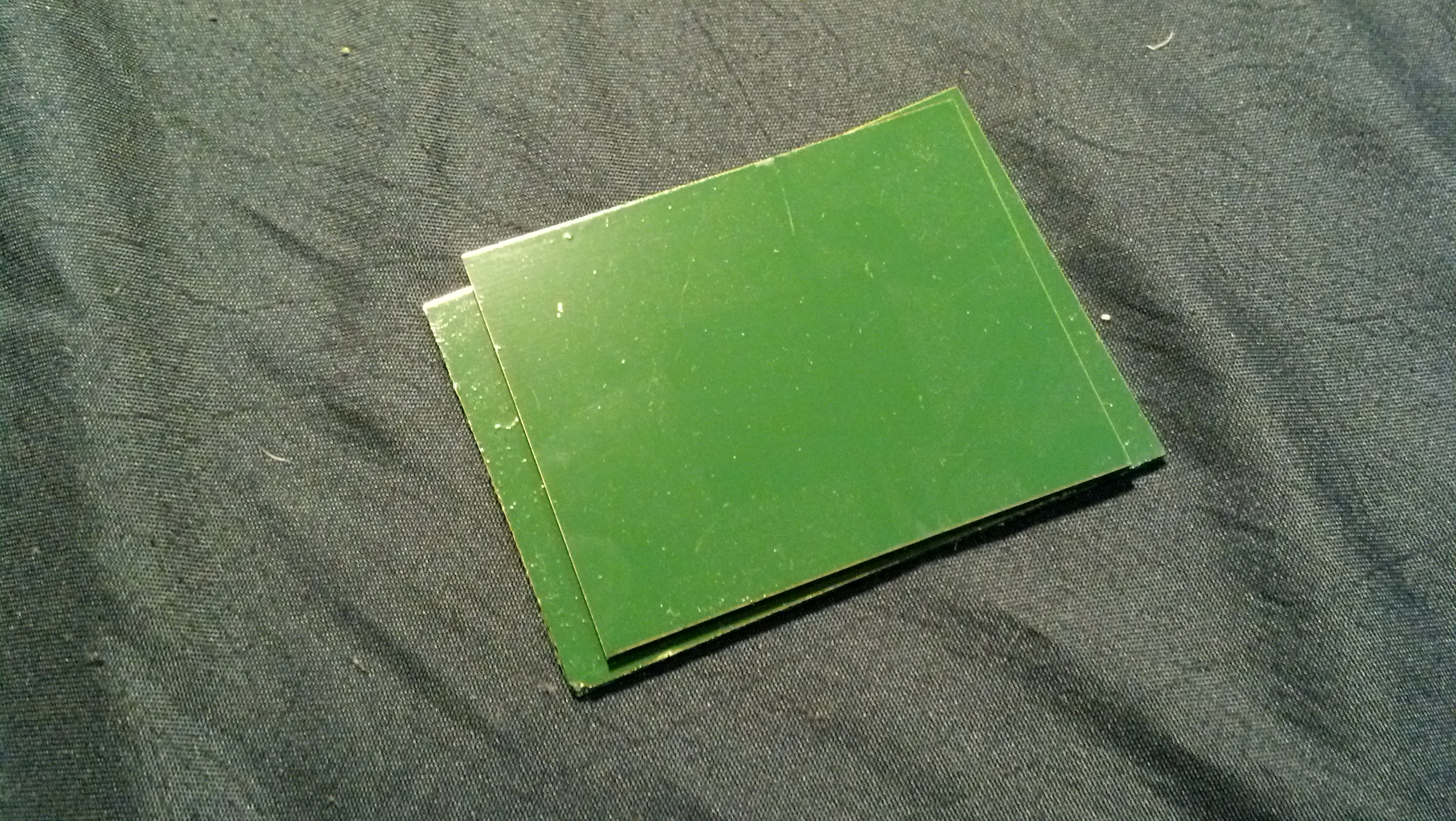
After designing the schematics and laying out my PCB in Eagle, I created my PCB. I used a mask technique described in a couple guide online, which I will redescribe here. First, I cut my copper clad sheet and cleaned it with acetone and steel wool. Then, I coated it in 2-3 coats of spray paint.
I first used green-painted copper clad sheet but later used white-painted sheet after I attempted to etch the former with some bunk etching solution.
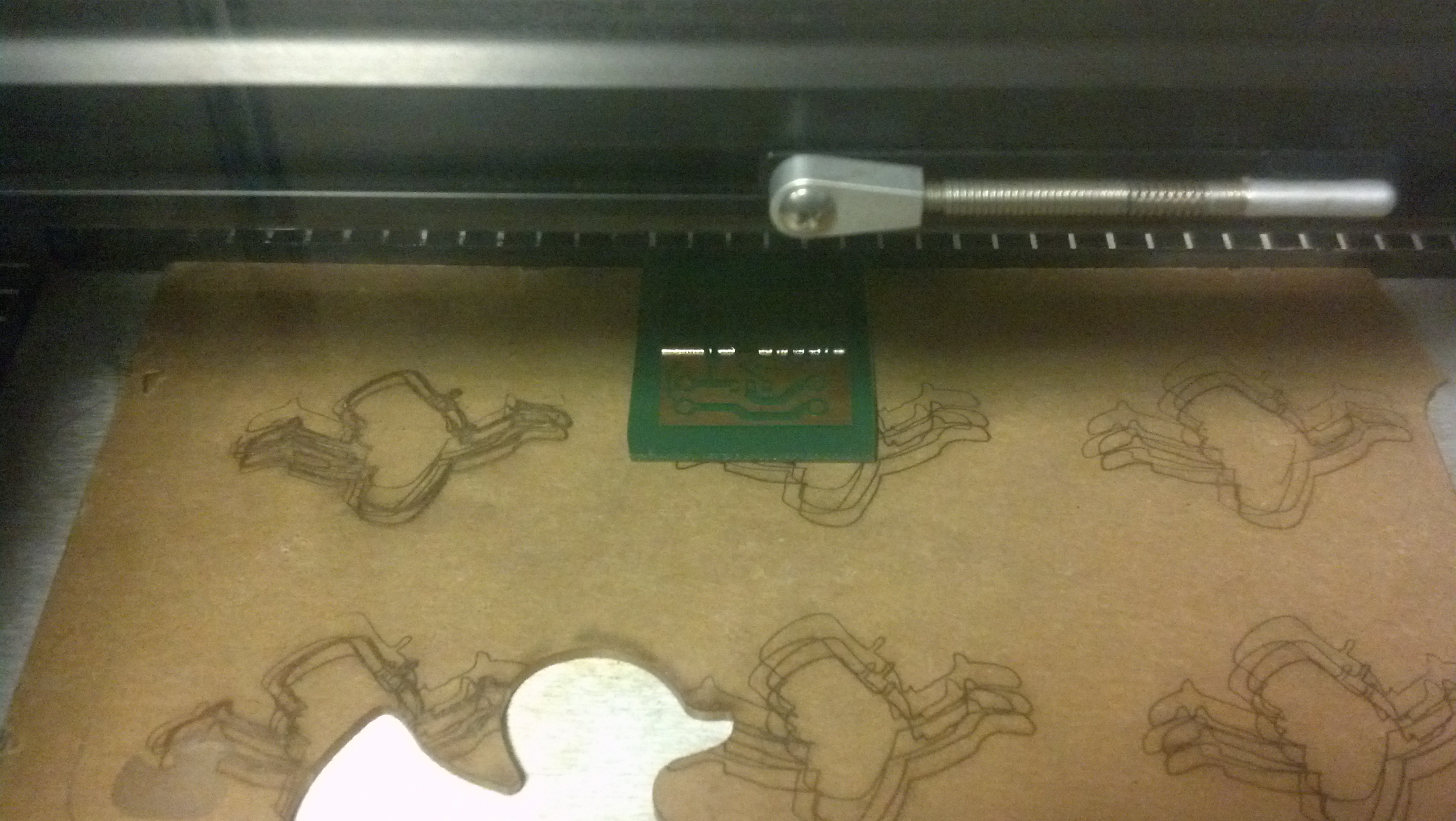
Next, I used a laser cutter to blast off the paint in areas I wanted to etch.
lazors
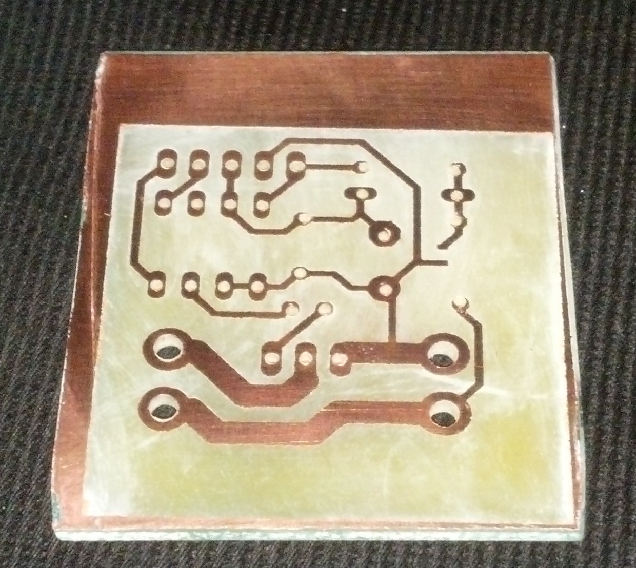
Finally, I etched the board like normal and used acetone to remove the paint.
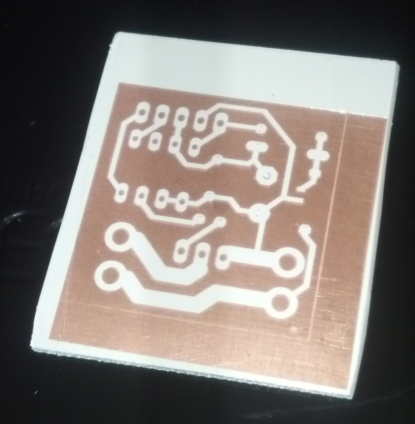
Here’s the circuit I finally etched, with white spray paint mask.
After I etched the board and acetoned off the paint, I drilled holes in the PCB.
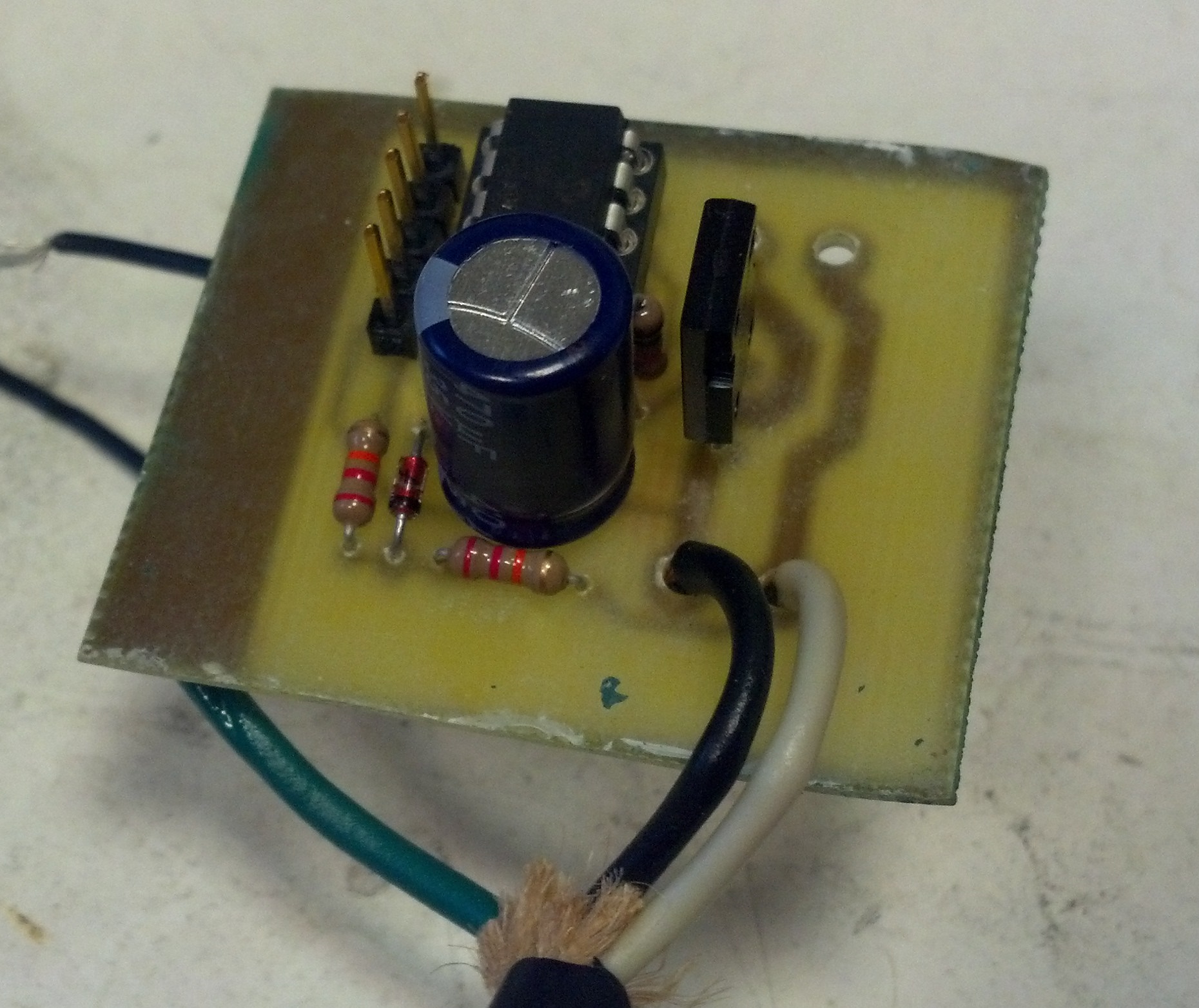
After etching, I populated the board, debugged it, powered it on, and programmed it. Don’t touch this! Mains is exposed here in bare copper. I plan to encase this for safety.
Software and Debugging
Next, I debugged and programmed the system. The microcontroller pin connected to the circuit through a 22k resistor is for zero crossing detection. I was hoping to use the sleep function of the microcontroller to put the microcontroller in a low power state until a change was detected on this pin, indicating zero crossing, but I realized the microcontroller had no memory between resets, so I could not implement this while also implementing a fade effect, which requires a counter that passes its state cycle after cycle. Instead, I just looped my program until a change was detected on the pin.
For simplicity, I designed with entirely through-hole components, except for my zener because I could not find low enough current zener that was through-hole. The two black wires were temporarily attached for debugging.
As indicated before, debugging was difficult because I could only measure differential measurements with my grounded oscilloscope. Initially, this proved to be ineffective because the oscilloscope could not provide volt-scale resolution on differential measurements while reading 120V measurements. I attempted to use a high voltage differential probe, but this also proved ineffective for measurements on the order of volts. Ultimately, I connected my circuit to mains through an isolation transformer, allowing me to probe the 0V and 5V nodes directly.
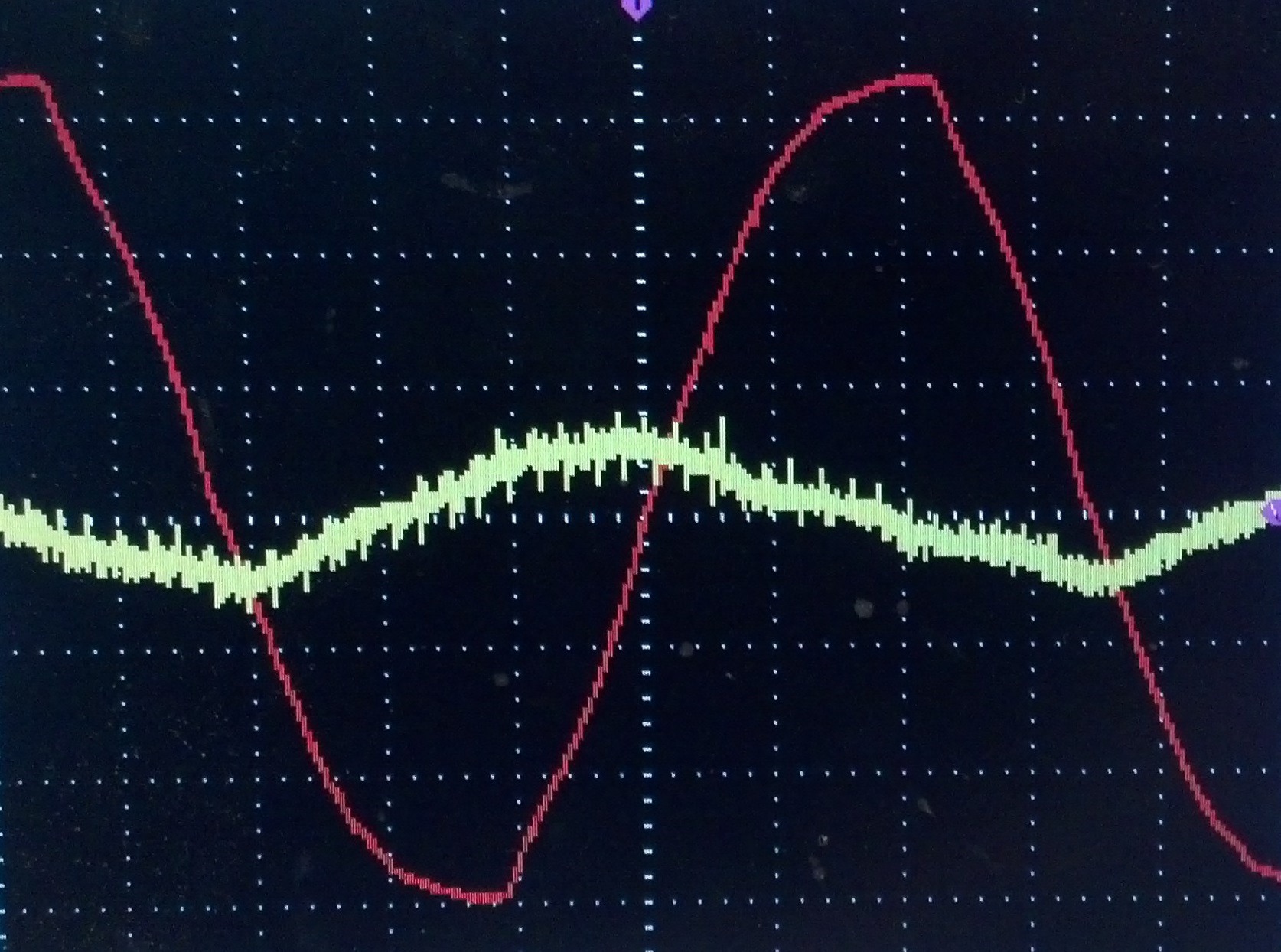
This oscilloscope reading shows two signals of different scales. Red is neutral measured relative to hot, at 50V/div. Yellow is the 5V power supply, measured at 20mV/div. Yellow has a ripple roughly 30mV peak to peak. During one half cycle, the capacitor recharges, and during the other, it discharges.
Check it out in action!
You can see in the video above that I shrunk the capacitor per my above note about sizing.