Following up my last post, I took another Introduction to Robotics class last semester, but this time it was the Mechanical Engineering department’s 2.12, which goes into more depth on the modelling and control of robotic mechanisms. See my previous post for a quick comparison of the classes.
Instead of exploring an environment and building a structure out of blocks, the final project for 2.12 was a little more constrained. The final project was the World Cup of robotics, a soccer competition to be played by the robots of the class. The class was divided into several groups, each representing a nation, and each group fielded a goalie robot and a kicker robot. A team of three other undergrads and me, dubbed “Team Kicking and Screaming” built the kicker robot for our nation.
Here, you can see our final robot in action. The robot uses data from a camera system to predict the ball’s motion. With this model, it then calculates the point in time and space at which the ball will intersect the workspace of the robot. When the ball is close enough, the robot starts a kicking trajectory such that the shoe will meet the ball at this point in time.
In order to implement this behavior, we wrote several software modules. These included a module for accessing the camera system, a module for predicting the path of the ball, and a module for inverse kinematics and motor control, among others.
For vision, the 2.12 TAs set up a computer to extract the ball coordinates from a ceiling-mounted camera using techniques we studied in an earlier lab assignment. The machine published these coordinates to a TCP server with updates promised roughly 60 times a second. We first wrote software to poll this server and to perform calculations with the data.
Next, we got to work with ball trajectory tracking. We were writing software at the same time as the TAs were setting up their vision software, so we weren’t able to immediately test different models of rolling ball motion using real data. With this in mind, I deliberately left the model as a parameter that could be supplied by the user, and I used the curve_fit method of SciPy’s Optimize module to fit the data to whatever model was supplied. This method uses the Levenberg–Marquardt algorithm for curve fitting, which can be applied even for non-linear curve fitting.
Written before the camera system was set up, a piece of our software software generated the following demo image. Upon being fed coordinates that represent sampled locations of the ball, plotted in blue, the software adjusted parameters to fit a trajectory model, and it plotted the calculated trajectory in green. The red line is the software’s prediction of the future path of the ball if it remains on this trajectory. The sample points were broadcast from a server hosted locally and were deliberately spaced far apart for ease of debugging, but the actual data would be more dense spatially.
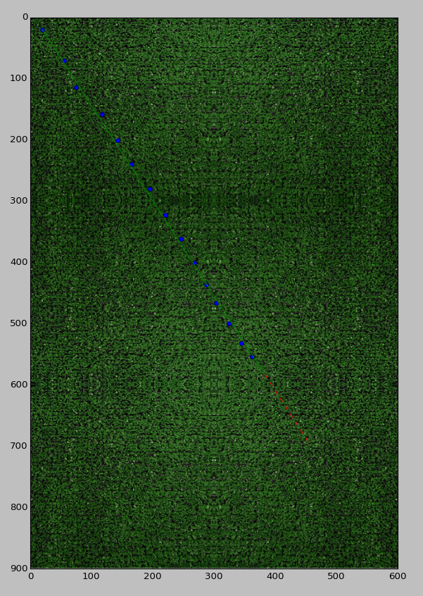
Our software fit the above trajectory to the blue points as they were published. The axes are measured in pixels; the resolution of the field is roughly 2.5px/in. Once built, the actually field was a little smaller, and ball coordinates were published much more densely.
Once the field and camera system was set up and we observed the movement of the ball, it became apparent to us that the a good model of ball motion could indeed be nonlinear. As the ball slowed, the general curvature of its trajectory often increased. More significantly though, being a buckyball-shaped soccer ball, the ball would wobble from side to side as it landed on different faces of its surface. This motion was on the order of inches.
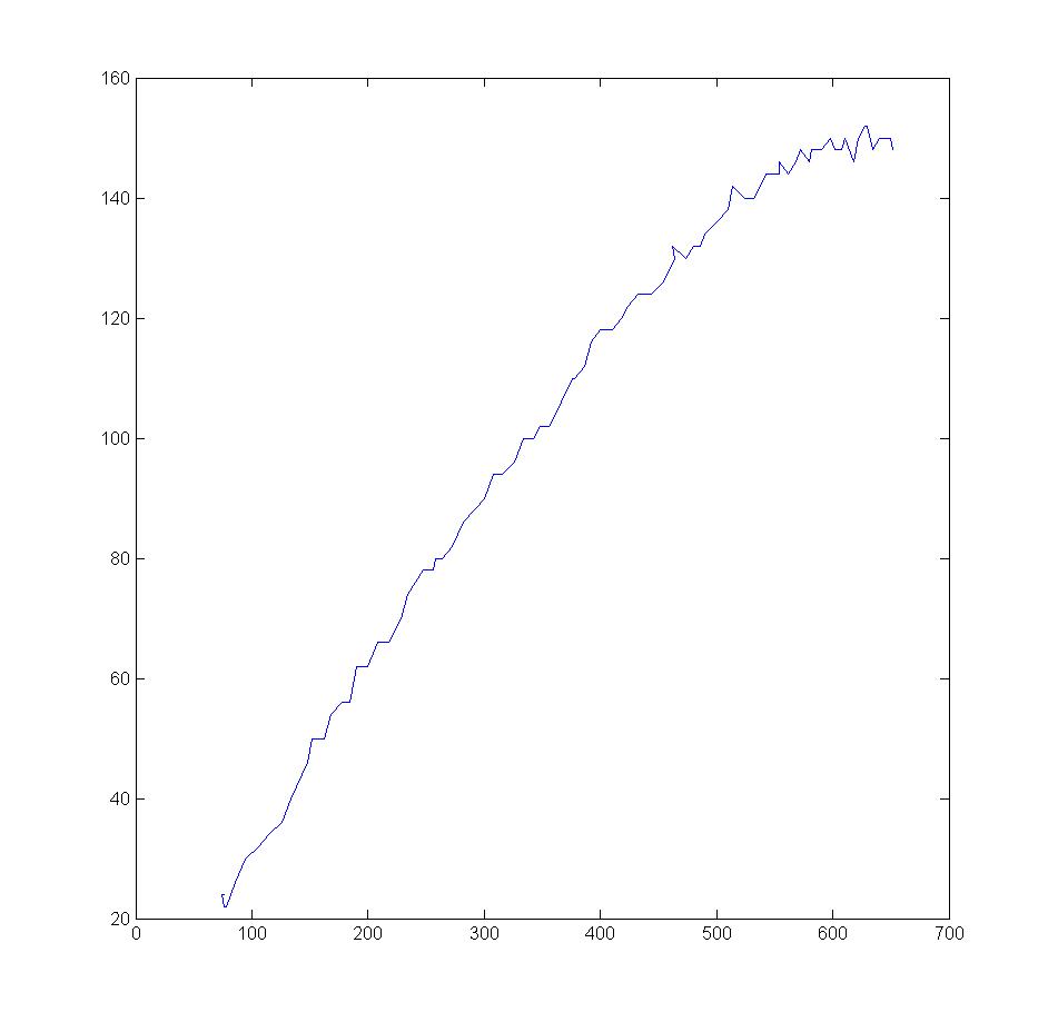
This plot of a ball’s motion over the field coordinates, captured from the field vision system, demonstrates the wobbliness of the ball’s motion as it slows down. The ball entered from the lower left and rolled to the upper right. Both axes are in pixels at roughly 3.5px/in. This plot is deliberately compressed to make the curvature more apparent.
Luckily, as the project progressed, it became apparent that they intended to roll the ball at a higher speed than what we were initially testing. At higher speeds, the wobbling effect was diminished, and we were able to use a relatively simple model of a rolling ball with rolling resistance.
Once we had this ball trajectory, we wanted our robot to be able to predict at what point the ball would intersect the workspace of our robot. At this point, unsure of what ball trajectory model we would use, we were faced with the problem of finding the intersection of two arbitrary curves: the trajectory of the ball, and the perimeter of the workspace of our robot.
Our solution was to discretize each curve as a finite number of line segments and then iterate through them until an intersection was found–this way, we could make a trade-off between the spatial resolution of the intersection point and the amount of time to compute the point. This strategy finds the intersection point, if there is one, as long as the line segment lengths are small compared to how far the path can diverge from a straight line approximation over a single discretization step. In our case, the inertia of the ball limits how far its path could diverge from a straight line.
It turns out there aren’t many computational geometry modules available in Python, so I ended up writing my own to evaluate whether two line segments intersect. I’d be happy to hear if I overlooked something, so let me know.
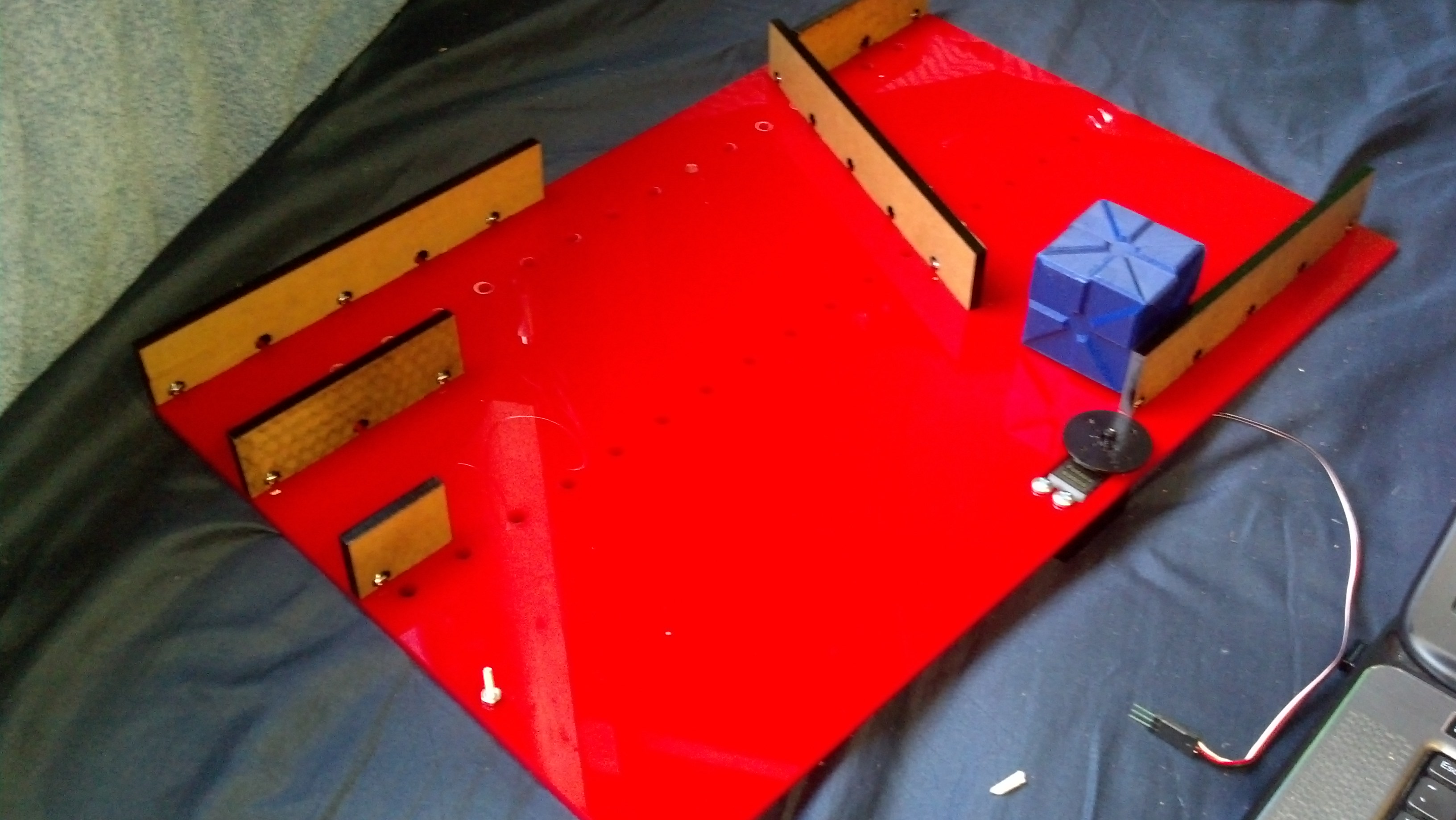
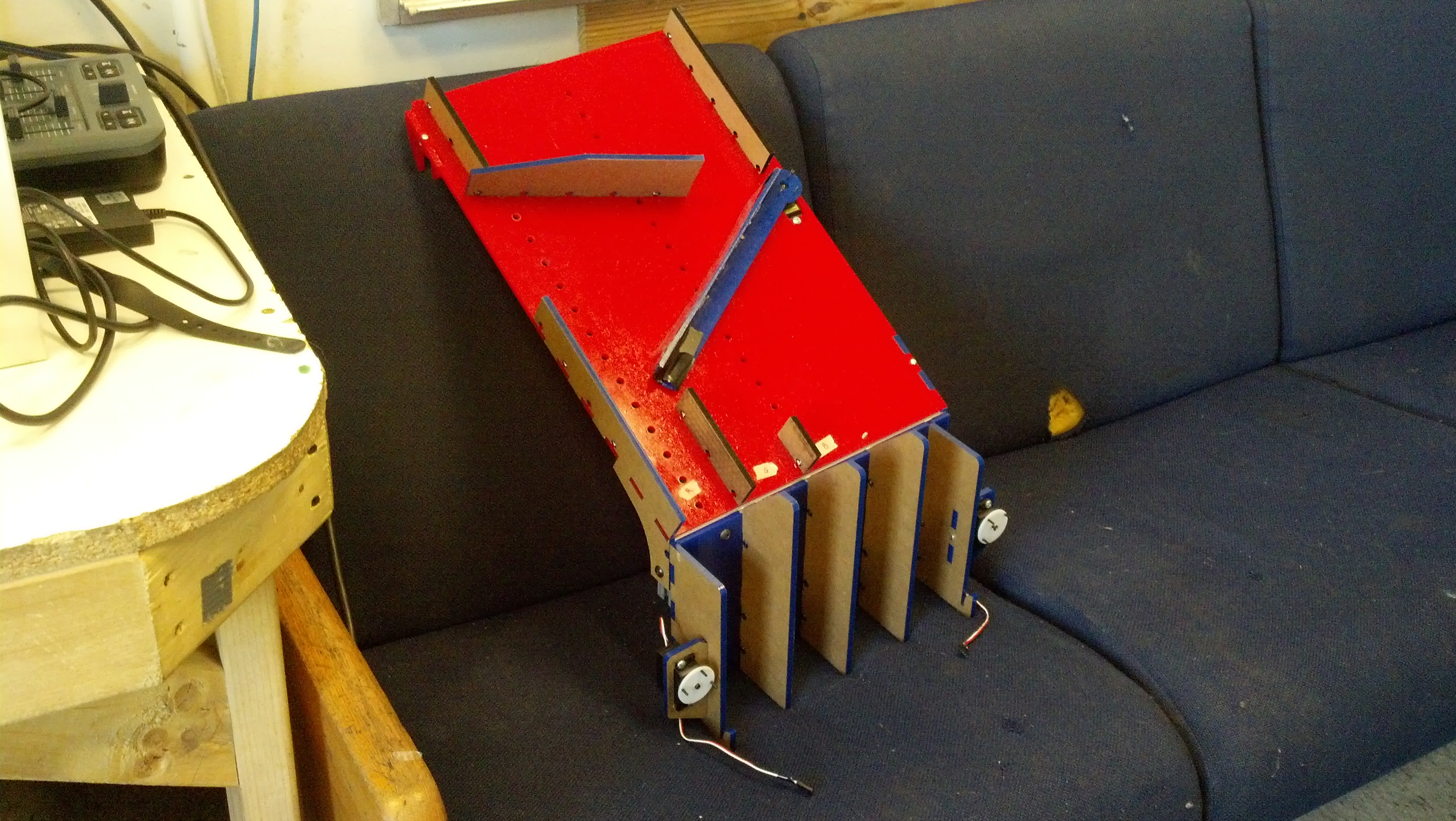
The other members of my team developed the hardware for the robot, though I waterjetted some parts. The result of their design was this super kickass leg, as you can see from these renderings.
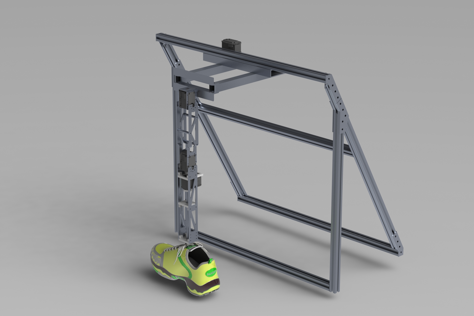
The frame of the robot attaches to a baseplate on the field while the leg terminates in a shoe to interface with the ball.
Once we developed the design for our robotic manipulator, we performed wrote software to perform inverse kinematics with the parameters for our robot. With this kinematic model available, we wrote software so that that our leg would follow a trajectory, ending at the time and space when the ball intersected our workspace.
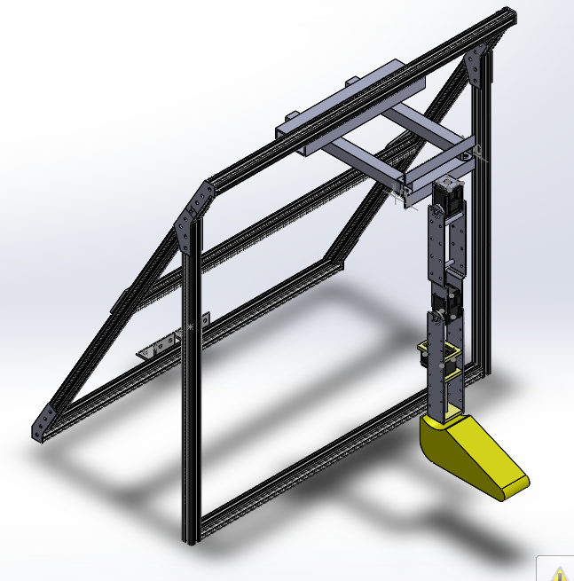
The lowest motor in this rendering adjusts the yaw of the ankle of the robot. Above this is a motor for controlling the angle of the knee, and above this is a motor for controlling the angle of the hip. The entire leg can move side-to-side, tracing out a semi-circle, using the driven parallel linkage between the hip and the frame.
Here’s the github repo for our code, which might be helpful for future teams. We wrote the majority of our code in Python with SciPy for curve fitting; and we used MATLAB and matplotlib for graphs.